11.1 Application

To apply EFA we will use the statsmodels package, which you already know from the previous sessions. Its factor analysis tools live in statsmodels.multivariate.factor, and you can read through the official documentation for further details.

When performing EFA, our objective is to find the optimal number of factors that effectively explain the relationships among a set of observed variables. The main steps involved in this process are:

1. Determining the number of factors

2. Interpreting the initial factor loadings

3. Rotating factors for better interpretation

A factor is a latent variable summarizing the shared variance among observed variables. EFA aims to reduce the dimensionality by retaining fewer factors than observed variables. Factor loadings are the relationship between each observed variable and the factor. For orthogonal factors (when factors are not correlated), these loadings can be viewed as correlations. High loadings indicate strong associations.

Creating the Data¶

To demonstrate EFA, we will create a simulated dataset containing 9 variables (items). Three items each cover one underlying factor, with the items being:

• Q1: In the past two weeks, how often have you felt down, depressed, or hopeless?

• Q2: How often have you lost interest or pleasure in activities you used to enjoy?

• Q3: How often have you felt tired or had little energy over the last two weeks?

• Q4: How often have you felt nervous, anxious, or on edge in the past two weeks?

• Q5: In the past two weeks, how often have you found it difficult to relax?

• Q6: How often have you been easily annoyed or irritable in the past two weeks?

• Q7: How satisfied are you with your life as a whole?

• Q8: To what extent do you feel that your life is close to your ideal?

• Q9: In general, how happy are you with your current situation in life?

import numpy as np
import pandas as pd
import matplotlib.pyplot as plt
import seaborn as sns

# Simulate data
np.random.seed(42) # Set seed for reproducible results
n = 300 # Number of rows ("participants")

# Create the items (we assume three underlying factors with three items each)
D = np.random.normal(5, 1, n).reshape(n, 1) + np.random.normal(0, 0.5, (n, 3))
A = np.random.normal(4, 1, n).reshape(n, 1) + np.random.normal(0, 0.5, (n, 3))
LS = np.random.normal(6, 1, n).reshape(n, 1) + np.random.normal(0, 0.5, (n, 3))

# Create the df
data = np.hstack([D, A, LS])
columns = ['Q1', 'Q2', 'Q3', 'Q4', 'Q5', 'Q6', 'Q7', 'Q8', 'Q9']

df = pd.DataFrame(data, columns=columns)
df.head()

Inspecting the Data¶

Before conducting a factor analysis it is worthwhile to look at the correlation matrix of the data of interest.

ax = sns.heatmap(df.corr(), cmap="viridis", square=True, vmin=0, vmax=1)
ax.set_title("Correlation matrix");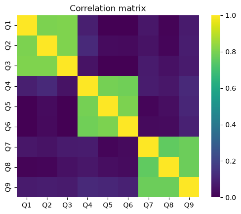

Here we can already see three blocks: items Q1-Q3, items Q4-Q6, and items Q7-Q9 each correlate highly among themselves, but only weakly with the items of the other blocks.

Determining the Number of Factors¶

Several approaches are possible to determine the number of factors. Here we apply the Kaiser criterion and select as many factors as there are eigenvalues > 1.

An eigenvalue of the correlation matrix is the amount of variance (measured in units of single items) captured by one direction in the data. Because each standardised item contributes exactly 1 unit of variance, a factor with an eigenvalue below 1 explains less than a single item does, which is why 1 is the natural cut-off. We can read these eigenvalues straight off the correlation matrix:

eigenvalues = np.sort(np.linalg.eigvalsh(df.corr()))[::-1]  # largest first
print(np.round(eigenvalues, 3))
print(f"\nNumber of eigenvalues > 1: {(eigenvalues > 1).sum()}")

[2.85  2.556 2.347 0.257 0.232 0.211 0.204 0.186 0.158]

Number of eigenvalues > 1: 3

Plotting them gives the familiar scree plot:

ax = sns.lineplot(x=range(1, len(eigenvalues) + 1), y=eigenvalues, marker="o")
ax.axhline(1, color="red", linestyle="--", label="Kaiser criterion")
ax.set(xlabel="Factor", ylabel="Eigenvalue")
ax.legend();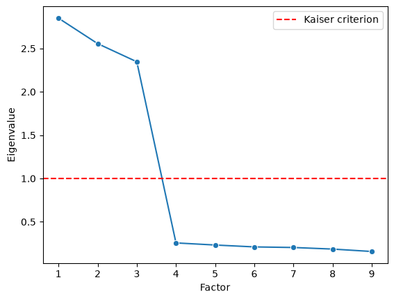

We can see that three factors have eigenvalues above 1 and we therefore choose a 3-factor solution for the final model.

Additional information: such a plot is called a scree plot, and we usually want to look for a “bend” in the plot. In this case, the bend corresponds to the same solution as the Kaiser criterion.

Fitting and Interpreting the Final Model¶

Before fitting the final model, one has to choose whether to use independent (orthogonal rotation) or correlated (oblique rotation) factors. In psychology, it most often has to be assumed that the constructs we measure are somewhat correlated and therefore an oblique rotation is often suitable. statsmodels offers several rotation methods, including the oblique oblimin, quartimin and promax.

We create a Factor object, set the number of factors and the estimation method (here Maximum Likelihood), fit it, and then apply the rotation:

from statsmodels.multivariate.factor import Factor

fa = Factor(df, n_factor=3, method="ml").fit()
fa.rotate("oblimin")

To interpret the model the factor loadings can be printed. The resulting matrix has three columns (factors) and nine rows (items).

loadings = pd.DataFrame(
    np.real_if_close(fa.loadings),   # the rotation returns a complex array
    index=df.columns,
    columns=[f"Factor {i}" for i in (1, 2, 3)],
)
loadings.round(2)

We can see that items Q1-Q3 load mostly onto one factor, items Q4-Q6 onto another, and items Q7-Q9 onto the third.

Note: factor loadings are similar to standardized regression coefficients, and variables with higher loadings on a particular factor can be interpreted as explaining a larger proportion of the variation in that factor.

To evaluate how good the model is one might look at the communalities. Communalities range from 0 to 1 and tell you the variance of each observed variable accounted for by all extracted factors combined. In statsmodels this is 1 minus the uniqueness (the share of an item’s variance that the factors do not explain):

communalities = pd.Series(1 - fa.uniqueness, index=df.columns, name="Communality")
communalities.round(3)

As the communalities are quite high for all variables we can conclude that the model fits the data well.