6.1 Multiple Linear Regression - Multivariate Statistics with Python

Multiple linear regression involves performing linear regression with more than one independent variable. As you may know, multiple regression with n predictors can be expressed as:

y_i = \beta_0 + \beta_1 x_{i1} + \beta_2 x_{i2} + \dots + \beta_k x_{in} + \epsilon_i

(1)

In this equation:

$\beta_0$ is the intercept, representing the expected value of $y$ when all $x$ -values (predictors) are 0.
$\beta_1$ represents the change in $y$ for a one-unit increase in $x_{i1}$ , while all other predictors are held constant.
The same interpretation applies to the other predictors, $\beta_2, \beta_3, ..., \beta_n$
$\epsilon_i$ represents the residual variance that is not explained by the model.

In Python, various methods and libraries are available for performing multiple regression. Some methods involve manual implementation, while others utilize libraries such as sklearn or statsmodels. For this example (and for many more models in the upcoming weeks), we will focus on using statsmodels.

As an example, let us consider the trees data set from the datasets package, which includes measurements of the girth, height, and volume of 31 felled black cherry trees.

Step 1: Importing the Libraries¶

import pandas as pd                   # Pandas to handle the data
from statsmodels.api import datasets  # Module for the data set
import statsmodels.formula.api as smf # Module for the regression

import seaborn as sns                 # Seaborn for simle plotting
import matplotlib.pyplot as plt       # Matplotlib to show the figure

Step 2: Loading and Preprocessing the Data¶

We will now import the “trees” dataset and convert the measurements from inches, feet, and cubic feet to meters and cubic meters (because no one likes imperial units). After that, we’ll view the first few rows of the dataset using the head() method.

# Load the "trees" dataset from R datasets
trees_data = datasets.get_rdataset('trees').data

# Convert units
trees_data['Girth']  = trees_data['Girth']  * 0.0254 # inches to meters
trees_data['Height'] = trees_data['Height'] * 0.3048 # feet to meters
trees_data['Volume'] = trees_data['Volume'] * 0.0283 # cubic feet to cubic meters

# Round to 3 decimal places
trees_data = trees_data.round(3)

# Display the first few rows of the dataset
print(trees_data.head())

   Girth  Height  Volume
0  0.211  21.336   0.291
1  0.218  19.812   0.291
2  0.224  19.202   0.289
3  0.267  21.946   0.464
4  0.272  24.689   0.532

Step 3: Visualizing the Data¶

Before we proceed with modeling, it is strongly recommended to visualize the data. Here it can, for example, guide us in determining whether linear regression is appropriate. We’ll use the pairplot() function from the seaborn package to create scatterplots for every pair of variables, and a histogram for each variable.

Additional information: In a Jupyter Notebook, we do not need the explicit plt.show(). However, it would always be needed in a normal Python script, so I put it here to avoid any potential confusion.

sns.pairplot(trees_data);
plt.show()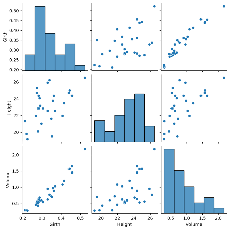

Based on the visual inspection, we see that there seems to be a strong linear relationship between the volume and girth of the trees, and a weaker relationship between the volume and the height.

Step 4: Fitting the Model¶

Next, we will create a multiple linear regression model with Volume as the dependent variable, and Girth and Height as the independent variables.

For this, we will use the ols() class from the statsmodels.formula.api module to build the model. The regression equation is specified in formula notation: response ~ predictor(s). In case of multiple predictors, they are separated by a + sign. Once a model is specified correctly, the fit() method can be used to fit the model, and the summary() method will then provide a detailed overview of the model results.

model = smf.ols(formula='Volume ~ Girth + Height', data=trees_data)
results = model.fit()
print(results.summary())

                            OLS Regression Results                            
==============================================================================
Dep. Variable:                 Volume   R-squared:                       0.948
Model:                            OLS   Adj. R-squared:                  0.944
Method:                 Least Squares   F-statistic:                     253.3
Date:                Wed, 12 Aug 2026   Prob (F-statistic):           1.17e-18
Time:                        12:23:52   Log-Likelihood:                 25.963
No. Observations:                  31   AIC:                            -45.93
Df Residuals:                      28   BIC:                            -41.62
Df Model:                           2                                         
Covariance Type:            nonrobust                                         
==============================================================================
                 coef    std err          t      P>|t|      [0.025      0.975]
------------------------------------------------------------------------------
Intercept     -1.6422      0.245     -6.698      0.000      -2.144      -1.140
Girth          5.2496      0.296     17.755      0.000       4.644       5.855
Height         0.0315      0.012      2.597      0.015       0.007       0.056
==============================================================================
Omnibus:                        0.872   Durbin-Watson:                   1.261
Prob(Omnibus):                  0.647   Jarque-Bera (JB):                0.912
Skew:                           0.300   Prob(JB):                        0.634
Kurtosis:                       2.412   Cond. No.                         359.
==============================================================================

Notes:
[1] Standard Errors assume that the covariance matrix of the errors is correctly specified.

Specifying a model with formula notation is useful, as it is identical to the syntax of the R programming language. If you are comfortable with either one, you can quickly switch between both programming languages.

# R code
model <- lm(Volume ~ Girth + Height, data = trees_data)
summary(model)

An alternative (and slightly more flexible) way of creating a regression model using statsmodels is to use the standard OLS class:

import statsmodels.api as sm

# Define dependent (y) and independent (X) variables
X = trees_data[['Girth', 'Height']]  # Select predictors
X = sm.add_constant(X)               # Add constant for the intercept
y = trees_data['Volume']             # Response variable

model = sm.OLS(y, X)
results = model.fit()

This can be useful if you need special control over your design matrix (e.g., custom transformations or programmatic workflows), but requires the extra step of creating it yourself (which also includes to manually add the intercept term). Thus, we will mostly use the intially shown syntax, which under the hood uses the patsy package to convert formulas and data to the matrices that are used in model fitting.

Step 5: Interpreting the Model Outputs¶

The regression summary provides important information about the model:

Intercept ( $\beta_0$ ): This is the predicted value of Volume when Girth and Height are both zero.
Girth ( $\beta_1$ ): This represents the change in Volume for a one-unit increase in Girth, assuming Height remains constant.
Height ( $\beta_2$ ): This represents the change in Volume for a one-unit increase in Height, assuming Girth remains constant.

Each coefficient includes:

Standard error: Measures the accuracy of the coefficient estimate.
t-value: Tests the hypothesis that the coefficient is different from zero.
p-value: A small p-value suggests that the predictor variable is statistically significant.

R-squared and Adjusted R-squared

R-squared: Indicates the proportion of variance in the dependent variable explained by the model. It increases with more predictors, even if they don’t improve the model.
Adjusted R-squared: Adjusts for the number of predictors, penalizing for adding unnecessary predictors, and is more reliable for evaluating model performance.

F-statistic

The F-statistic compares the fit of the model to a model with no predictors. A large F-statistic and a low p-value indicate that the independent variables have real predictive power.

Step 6: Making Predictions¶

Now that we have a fitted model, we can predict a volume given some (unseen) girth and height. To do this, we use the predict() method:

X_predict = pd.DataFrame({'Girth': [0.3, 0.4, 0.5],
                   'Height': [20, 21, 22]})
prediction = results.get_prediction(X_predict)

for i in range(len(X_predict)):
    print(f"Predicted volume for a girth of {X_predict['Girth'].iloc[i]} and a height of {X_predict['Height'].iloc[i]} is: {prediction.predicted_mean[i]} m³")

Predicted volume for a girth of 0.3 and a height of 20 is: 0.5624568769459972 m³
Predicted volume for a girth of 0.4 and a height of 21 is: 1.1189061488332266 m³
Predicted volume for a girth of 0.5 and a height of 22 is: 1.6753554207204557 m³