To demonstrate multilevel regression models, we use the sleepstudy dataset from statsmodels. This is a well-known dataset in the field of mixed-effects modeling often used to illustrate the effects of sleep deprivation on cognitive performance. It contains measurements from a study on reaction times of 18 participants under sleep deprivation conditions over a period of 10 days and contains the following variables:
Reaction- the reaction time in milliseconds, which serves as the outcome variableDays- the number of days the participant has been sleep-deprived, ranging from 0 to 9Subject- A unique identifier for each participant, allowing for random effects in the model
# Load packages
import numpy as np
import pandas as pd
import statsmodels.api as sm
import statsmodels.formula.api as smf
import seaborn as sns
import matplotlib.pyplot as plt

# Load dataset
data = sm.datasets.get_rdataset("sleepstudy", "lme4").data
print(data.head())
Reaction Days Subject
0 249.5600 0 308
1 258.7047 1 308
2 250.8006 2 308
3 321.4398 3 308
4 356.8519 4 308
Plot the data
First, we plot a regression line through all data points, ignoring the nesting of individual subjects observations:
sns.lmplot(x='Days', y='Reaction', data=data)
plt.title("Combined regression");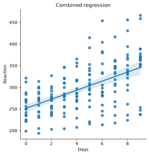
Next, let’s plot one for each subject, using Subject as the hue:
sns.lmplot(x='Days', y='Reaction', hue='Subject', data=data)
plt.title("Subject-specific regressions");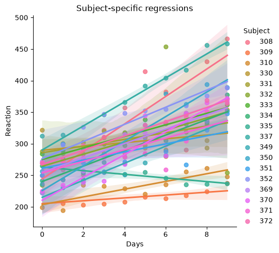
Reading the plot
By nesting participants observations, and plotting a regression line for each participant we recover patterns of variability that would have otherwise been be lost (or averaged out). Instead of treating each data point as an independent observation, we correctly group the dependent observations (nesting) with one an other, grouping by subject, and look at the variation across participants.
Intercept Variability:
The intercept represents the baseline Reaction time for each subject when Days = 0.
Some subjects have naturally higher baseline Reaction times, while others have lower ones. This variability suggests that individuals start at different points in terms of their Reaction times.
Slope Variability:
The slope represents the relationship between Days and Reaction time for each subject. It indicates how reaction times change as the number of days of sleep deprivation increases. Some subjects show a strong positive relationship (steep slope), meaning their Reaction times increase noticeably over Days. Others show little to no relationship.
Fitting multilevel regression models
In the following, we will create three multilevel regression models to provide an answer to the following research questions:
Q1: How much of the variation in
Reactionis due to differences betweenSubjects?Model 1: The unconditional model - This model includes no predictors and serves as a baseline to estimate how much of the variance in
Reactionis attributable to differences betweenSubjects(i.e., partitioning within-subject and between-subject variability).
Q2: What is the average effect of
DaysonReactionacross allSubjects?Model 2: The random intercept model - This model includes Days as a predictor at the within-subject level (Level 1). It assumes that all
Subjectshave the same slope (i.e., the effect ofDaysonReactionis constant across individuals), but allows eachSubjectto have their own baseline level ofReaction(random intercept).
Q3 and Q4: Does the effect of
DaysonReactionvary acrossSubject? Is there a relationship between an individual baseline reaction time (ReactionatDays = 0) and their rate of change inReactionover time (i.e., is there a correlation between intercept and slope)?Model 3: The random intercept and random slope model - This model extends Model 2 by allowing both intercepts and slopes to vary across
Subjects. It tests whether individualSubjectsdiffer in how theirReactionchanges over time (random slopes) and whether there is a correlation between an individual startingReactionlevel and their rate of change.
Model 1 - The unconditional model
Q1: How much of the variation in Reaction is due to differences between Subjects?
There is no predictor in the unconditional model. Here, we only estimate the intercept of Reaction and let it vary across the Level-2 units (Subject). The proportion of variance attributed to Level-1 units and Level-2 units can be estimated based on the estimated parameters in this model. In other words, this model can be used to compute the Intra-Class Correlation (ICC) coefficient, which indicates the strength of the effect of Subject (Level-2) on Reaction. More on ICC in the next sections.
# define and fit the unconditional model
model1 = smf.mixedlm("Reaction ~ 1",
                     data=data,
                     groups=data["Subject"])

# fit the model using the BFGS optimization method
model1_fit = model1.fit(method="bfgs")

# print the summary of the model
print(model1_fit.summary())
Mixed Linear Model Regression Results
========================================================
Model: MixedLM Dependent Variable: Reaction
No. Observations: 180 Method: REML
No. Groups: 18 Scale: 1958.8670
Min. group size: 10 Log-Likelihood: -952.1633
Max. group size: 10 Converged: Yes
Mean group size: 10.0
--------------------------------------------------------
Coef. Std.Err. z P>|z| [0.025 0.975]
--------------------------------------------------------
Intercept 298.508 9.050 32.985 0.000 280.770 316.245
Group Var 1278.324 12.009
========================================================
The summary provides two coefficients:
Intercept: The intercept (298.508) represents the estimated average reaction time in the dataset across all subjects, across all days (the unconditional model includes no predictors such as “days”). As indicated by the p-value, the intercept is significantly different from zero (p = 0.000). This is the fixed effect.Group Var: The variance of the random intercept is 1278.324. This value indicates how much individual subjects vary in their average reaction times at baseline. This is the random effect.
Intraclass Correlation Coefficient (ICC)
There is no included function to get the ICC. However, we can quickly code it ourselves:
# create function to calculate ICC
def calculate_icc(results):
    icc = results.cov_re / (results.cov_re + results.scale)
    return round(icc.values[0, 0], 4)

# call the function with your fitted model to calculate ICC
calculate_icc(model1_fit)np.float64(0.3949)An ICC of 0.39 indicates that 39% of the variance in Reaction is due to inter-individual differences.
Model 2 - The random intercept model
Q2: What is the average effect of Days on Reaction across all Subjects?
We now add the variable Days as predictor for Reaction. By estimating the average (fixed) slope, this model will inform about the average relationship between Days and Reaction. In this model, there is a predictor Days at Level-1 (individual), random intercepts and constant slopes across Level-2 units (Subject).
# define and fit the random intercept model
# this model includes "days" as a predictor at level 1
model2 = smf.mixedlm("Reaction ~ Days",
                     data=data,
                     groups=data["Subject"])

# fit the model using the BFGS optimization method
model2_fit = model2.fit(method="bfgs")

# print summary
print(model2_fit.summary())
Mixed Linear Model Regression Results
========================================================
Model: MixedLM Dependent Variable: Reaction
No. Observations: 180 Method: REML
No. Groups: 18 Scale: 960.4568
Min. group size: 10 Log-Likelihood: -893.2325
Max. group size: 10 Converged: Yes
Mean group size: 10.0
--------------------------------------------------------
Coef. Std.Err. z P>|z| [0.025 0.975]
--------------------------------------------------------
Intercept 251.405 9.747 25.794 0.000 232.302 270.508
Days 10.467 0.804 13.015 0.000 8.891 12.044
Group Var 1378.176 17.156
========================================================
The summary provides three coefficients:
Intercept: The intercept (251.405) represents the estimated average reaction time at baseline (days = 0), across all subjects. This is significantly different from zero (p = 0.000).Days: The average relationship (slope) betweenDaysandReaction. This indicates that, on average, for each additional day, the reaction time increases by approximately 10.47 ms. This is significantly different from zero (p = 0.000).Group Var: The variance of the random intercept is about 1378. This value indicates how much individual subjects vary in their average reaction times at baseline. A higher variance suggests greater variability among subjects’ intercepts, meaning individual differences play a significant role in determining baseline reaction times.
Model 3 - The random intercept and random slope model
Q3: Does the effect of Days on Reaction vary across Subject?
Q4: Is there a relationship between an individual baseline reaction time (Reaction at Days = 0) and their rate of change in Reaction over time (i.e., is there a correlation between intercept and slope)?
Model 3 includes the Days predictor (level 1), a random intercept, and a random slope. This model estimates the variance of the slope and determines whether the relationship between Days and Reaction varies across individuals (Subject). We now additionally provide re_formula as a one-sided random effects formula defining the variance structure of the model. This specifies that random effects are modeled as a function of Days, allowing each subject to have its own intercept and slope.
# define the random intercept and random slope model
# model includes "days" as a predictor at level 1
model3 = smf.mixedlm("Reaction ~ Days",
                     data=data,
                     groups=data["Subject"],
                     re_formula="~Days")        #random effects

# fit the model
model3_fit = model3.fit(method="bfgs")

# print summary
print(model3_fit.summary())
Mixed Linear Model Regression Results
==============================================================
Model: MixedLM Dependent Variable: Reaction
No. Observations: 180 Method: REML
No. Groups: 18 Scale: 654.9405
Min. group size: 10 Log-Likelihood: -871.8141
Max. group size: 10 Converged: Yes
Mean group size: 10.0
--------------------------------------------------------------
Coef. Std.Err. z P>|z| [0.025 0.975]
--------------------------------------------------------------
Intercept 251.405 6.825 36.838 0.000 238.029 264.781
Days 10.467 1.546 6.771 0.000 7.438 13.497
Group Var 612.096 11.881
Group x Days Cov 9.605 1.821
Days Var 35.072 0.610
==============================================================
We now get additional coefficients (Group x Days Cov and Days Var):
Days Var: Represents the variance of the random slopes for theDaysvariable acrossSubject. Some subjects have a steeper increase in reaction time over days, while others may have a slower or negligible increase. A high variance thus indicates more variability among individuals in how their reaction times change over days.Group x Days Cov: Describes the covariance between the random intercept and the random slope forDays. The positive covariance indicates that subjects with higher baseline reaction times (intercepts) also tend to have larger increases in reaction time over days (steeper slopes).