Now, let’s apply path modeling to the real-world example. As explained in the introduction, we will investigate the relationships between physical health, functional health, and subjective health, as proposed by Whitelaw and Liang (1991).
We’ve formulated the following hypotheses for our investigation:
Physical health influences functional health, which, in turn, predicts subjective health.
Physical health directly affects subjective health.
Based on these hypotheses, we structure the relationships into the following diagram:
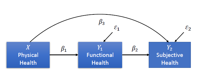
Variables
Physical Health (): The number of illnesses experienced in the last 12 months (higher values indicate poorer physical health).
Functional Health (): The sum score of the SF-36 questionnaire, which measures functional health.
Subjective Health (): Self-reported subjective health, reflecting how individuals perceive their overall health.
Loading the data
The data is provided in the book. As in the previous session, we can either load it from the local files (if you downloaded the entire book), or from the GitHub link. We will again use the second version as this would also work in Google Colab:
import pandas as pd
import semopy
import matplotlib.pyplot as plt

df = pd.read_csv("https://raw.githubusercontent.com/mibur1/psy111/main/book/statistics/5_Path_Modelling/data/data.txt", sep="\t")
print(df.head())
1 1.1 0 13 1.2 1.3 1.4
0 1 1 7 15.5 1.0 1.0 1.0
1 1 1 3 19.0 1.0 1.0 1.0
2 1 1 6 20.0 1.0 1.0 1.0
3 1 2 10 20.5 1.0 1.0 1.0
4 1 1 7 22.5 1.0 1.0 1.0
We can see that the columns to not have names, so we assign them based on knowledge we have about the data:
df.columns = ["SubjHealth","SubjHealthChange", "PhysicHealth", "NrDoctorApp", "FunctHealth", "FunctHealth1", "FunctHealth2"]
print(df.head())
SubjHealth SubjHealthChange PhysicHealth NrDoctorApp FunctHealth \
0 1 1 7 15.5 1.0
1 1 1 3 19.0 1.0
2 1 1 6 20.0 1.0
3 1 2 10 20.5 1.0
4 1 1 7 22.5 1.0
FunctHealth1 FunctHealth2
0 1.0 1.0
1 1.0 1.0
2 1.0 1.0
3 1.0 1.0
4 1.0 1.0
Great, the DataFrame now looks like it is ready for use! We can continue with defining and fitting the model:
# Define the model
model = semopy.Model("""
                     SubjHealth ~ PhysicHealth + FunctHealth
                     FunctHealth ~ PhysicHealth
                     """)

# Fit the model to our data and estimate parameters
info = model.fit(df)
print(info)
Name of objective: MLW
Optimization method: SLSQP
Optimization successful.
Optimization terminated successfully
Objective value: 0.000
Number of iterations: 14
Params: -0.095 0.876 -0.096 0.172 0.432
We can then inspect the results:
estimates = model.inspect(std_est= True)
print(estimates)
lval op rval Estimate Est. Std Std. Err z-value \
0 FunctHealth ~ PhysicHealth -0.096184 -0.451359 0.004686 -20.527585
1 SubjHealth ~ PhysicHealth -0.094898 -0.244325 0.008330 -11.392426
2 SubjHealth ~ FunctHealth 0.876182 0.480711 0.039090 22.414663
3 FunctHealth ~~ FunctHealth 0.171521 0.796275 0.005977 28.696690
4 SubjHealth ~~ SubjHealth 0.431653 0.603198 0.015042 28.696690
p-value
0 0.0
1 0.0
2 0.0
3 0.0
4 0.0
This output provides a detailed breakdown of the parameter estimates from the model.
Or the fit statistics:
stats = semopy.calc_stats(model)
print(stats)
DoF DoF Baseline chi2 chi2 p-value chi2 Baseline CFI \
Value 1 4 0.000113 0.991515 1207.802947 1.000831
GFI AGFI NFI TLI RMSEA AIC BIC LogLik
Value 1.0 1.0 1.0 1.003322 0 10.0 37.033554 6.866405e-08
Finally, we can also visualise the model:
semopy.semplot(model, "figures/health.png", std_ests=True) # plot standardized estimatesAdditional information: If you want to visualise the model, you need to install Graphviz through pip (if you installed everything in the requirements.txt file you already have it). You then also need to install Graphviz as a normal program. On Windows, make sure to select the “Add Graphviz to PATH” option during the installation.
Model Output
Objective and Optimization
The first ouput we looked at after defining the model was info, which contains general information about the model fit:
Objective Function: Maximum Likelihood with Weights (MLW).
Optimization Algorithm: Sequential Least Squares Quadratic Programming (SLSQP).
Iterations: The model converged after 14 iterations.
Objective Value: 0.000, indicating that the model-implied covariance matrix closely reproduces the observed covariance matrix under the chosen estimation method.
Parameter Estimates
Functional Health ~ Physical HealthCoefficient: -0.096, SE: 0.0047, z: -20.527, p: < 0.001
Interpretation: Physical health (the number of illnesses) has a significant negative effect on functional health. More illnesses reduce functional health.
Subjective Health ~ Physical HealthCoefficient: -0.094, SE: 0.008, z: -11.39, p: < 0.001
Interpretation: Physical health has a significant negative effect on subjective health. More illnesses reduce subjective health.
Subjective Health ~ Functional HealthCoefficient: 0.876, SE: 0.039, z: 22.41, p: < 0.001
Interpretation: Functional health has a significant positive effect on subjective health. Higher functional health leads to better subjective health.
Standardized Coefficients
Standardized coefficients (Est.Std) allow us to compare the relative influence of each predictor on a common scale. They can be interpreted similarly to correlation coefficients in terms of strength and direction. However, unlike correlations, they represent model-implied directional associations that depend on the assumed causal structure of the model. By themselves, they do not establish causality, but quantify effects conditional on the specified paths.
Physical Health → Functional Health: -0.451 (strong negative effect).
Physical Health → Subjective Health: -0.244 (moderate negative effect).
Functional Health → Subjective Health: 0.481 (strong positive effect).
Variances
Functional Health ~~ Functional Health: Residual variance = 0.172 (p < 0.001). This represents the unexplained variance in functional health.Coefficient: 0.172, standardized coefficient: 0.796
Interpretation: The standardized Residual Variance indicates that approximately 80% of the individual variance in functional health remains unexplained by the model.
Subjective Health ~~ Subjective Health: Residual variance = 0.432 (p < 0.001). This represents the unexplained variance in subjective health.Coefficient: 0.432, standardized coefficient: 0.603
Interpretation: In this case, the standardized Residual Variance indicates that approximately 60% of the individual variance in subjective health remains unexplained by the model.
Model Evaluation
Fit Metrics
Chi-Square: 0.0001 (p = 0.9915).
CFI: 1.0008, TLI: 1.0033.
RMSEA: 0, GFI/AGFI: 1.0.
AIC: 10, useful for model comparison.
Interpretation of Model Fit
The model shows near-perfect fit indices. However, this should be interpreted with caution. The model has very few degrees of freedom (DoF = 1), meaning that global fit indices are not very informative in this context. In small or nearly just-identified models, it is common to observe extremely high fit values, including CFI and TLI values above 1 and RMSEA values close to zero.
Therefore, the excellent fit does not necessarily indicate overfitting, but rather reflects the simplicity and identification properties of the model.
Recommendation:
Model evaluation should focus primarily on parameter estimates and theoretical plausibility. External validation using an independent dataset can still be useful to assess generalizability.
Interpretation
Key Insights
Functional Health ~ Physical Health: Negative relationship; more illnesses (measured as higher score in physical health) lead to reduced functional health.Subjective Health ~ Physical Health: Negative relationship; more illnesses lead to poorer subjective health.Subjective Health ~ Functional Health: Positive relationship; higher functional health improves subjective health.
Implications
Mediation: The pattern of results is consistent with partial mediation by functional health. Physical health shows both a direct association with subjective health and an indirect association via functional health. A formal test of the indirect effect would be required to statistically confirm mediation.
Variance Explained: Functional health (20.6%), subjective health (39.7%). Other factors likely influence outcomes. These percentages represent R-squared values (explained variance) and are calculated as 1 minus the standardized residual variance.
Limitations
Limited Model Complexity: Due to the small number of variables and low degrees of freedom, global fit indices are of limited diagnostic value.
Self-reported Measures: Subjective health may suffer from biases (e.g., recall bias).
Large Unexplained Variance: Additional predictors (e.g., social factors) could enhance the model.