13.2 Centering Predictors

In regression modelling, a meaningful zero in a predictor variable is one for which the value zero has a sensible substantive interpretation. For example, a value of zero hours studied per day is, in principle, meaningful, whereas a value of zero years of age is not meaningful in a sample consisting only of adults.

In polynomial regression, the choice of where zero lies on the predictor scale is particularly important, because it directly affects the interpretation of lower-order coefficients. Centering a predictor variable by subtracting its mean often leads to clearer and more interpretable model parameters without changing the overall model fit.

Why center predictors?¶

Centering predictors in polynomial regression has several advantages:

• Improved interpretability
  The linear coefficient represents the rate of change of the outcome at the value of the predictor where $x = 0$. After centering, this corresponds to the mean of the predictor, which is often a more meaningful reference point than the original zero. It reduces the dependence of coefficient interpretation on arbitrary scale choices and avoids interpreting effects at values of the predictor that are not observed in the data.

• No change in model fit
  Centering does not affect predicted values, residuals, or the proportion of variance explained by the model. It only changes the numerical values and interpretation of the coefficients.

Centering study time¶

Consider the quadratic regression model

Without centering, the linear coefficient $\beta_1$ represents the rate of change of $y$ with respect to $x$ when $x = 0$. If zero is not a meaningful or observed value of the predictor, this interpretation is of limited practical value.

By centering the predictor, we redefine the zero point of the scale such that $x = 0$ corresponds to the mean of the predictor. As a result, $\beta_1$ is interpreted as the rate of change of the outcome at the average value of the predictor.

We use the same simulated data as before:

import numpy as np
import seaborn as sns
import statsmodels.api as sm
from matplotlib import pyplot as plt
from sklearn.preprocessing import PolynomialFeatures

# Simulate the data
np.random.seed(69)
study_time = np.random.uniform(2, 15, size=500)
h = 11   # location of the peak
k = 80   # maximum grade (without noise)
grades = -(k / (h**2)) * (study_time - h)**2 + k + np.random.normal(0, 8, study_time.shape)
grades = np.clip(grades, 0, 100) # ensure we only have grades between 0 and 100

Centering is achieved by subtracting the mean of the predictor from each observation:

study_time_centered = study_time - np.mean(study_time)

We then fit the centered quadratic model:

poly_features = PolynomialFeatures(degree=2, include_bias=True)
study_time_centered_features = poly_features.fit_transform(study_time_centered.reshape(-1, 1))

model_fit = sm.OLS(grades, study_time_centered_features).fit()

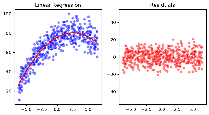
And visualise the model and residuals:

x_predict = np.linspace(study_time_centered.min(), study_time_centered.max(), 500)
x_predict_poly = poly_features.transform(x_predict.reshape(-1, 1))

predictions = model_fit.predict(x_predict_poly)
residuals = model_fit.resid

fig, ax = plt.subplots(1, 2, figsize=(8,4))

sns.scatterplot(x=study_time_centered, y=grades, color='blue', alpha=0.5, ax=ax[0])
ax[0].plot(x_predict, predictions, color='red', linewidth=2)
ax[0].set(title='Linear Regression')

sns.scatterplot(x=study_time_centered, y=residuals, color='red', alpha=0.5, ax=ax[1])
ax[1].axhline(0, linestyle='--')
ax[1].set(title="Residuals", ylim=(-55, 55));

print(model_fit.summary())

                            OLS Regression Results                            
==============================================================================
Dep. Variable:                      y   R-squared:                       0.802
Model:                            OLS   Adj. R-squared:                  0.801
Method:                 Least Squares   F-statistic:                     1007.
Date:                Wed, 12 Aug 2026   Prob (F-statistic):          1.50e-175
Time:                        12:24:10   Log-Likelihood:                -1714.2
No. Observations:                 500   AIC:                             3434.
Df Residuals:                     497   BIC:                             3447.
Df Model:                           2                                         
Covariance Type:            nonrobust                                         
==============================================================================
                 coef    std err          t      P>|t|      [0.025      0.975]
------------------------------------------------------------------------------
const         75.5318      0.487    155.109      0.000      74.575      76.489
x1             3.5570      0.093     38.402      0.000       3.375       3.739
x2            -0.6888      0.027    -25.493      0.000      -0.742      -0.636
==============================================================================
Omnibus:                        2.570   Durbin-Watson:                   2.050
Prob(Omnibus):                  0.277   Jarque-Bera (JB):                2.125
Skew:                          -0.007   Prob(JB):                        0.346
Kurtosis:                       2.681   Cond. No.                         26.3
==============================================================================

Notes:
[1] Standard Errors assume that the covariance matrix of the errors is correctly specified.

Interpretation¶

• Intercept
  The intercept represents the expected grade for a student with average study time. In this example, the predicted grade at the mean study time is 75.5%.

• Linear term
  The linear coefficient represents the instantaneous rate of change of grade with respect to study time at the mean study time. The positive value indicates that, at the average amount of studying, additional study time is still associated with increasing grades.

• Quadratic term
  The negative quadratic coefficient confirms an inverted U-shaped relationship between study time and grades, indicating diminishing and eventually negative returns at higher study times.

• Model fit
  Centering the predictor does not change the explained variance, fitted values, or residuals of the model. It only alters the numerical values and interpretation of the regression coefficients.