To fit regression splines, we continue with the same data as in the previous section. Again, we want to predict wage from age in the Mid-Atlantic Wage Dataset.
import numpy as np
import matplotlib.pyplot as plt
import seaborn as sns
import patsy
import statsmodels.api as sm
from ISLP import load_data

# Load the data
df = load_data('Wage')
Fitting piecewise linear splines
Similar to fitting a stepwise function, we first need to create the design matrix for our transformed predictor age. This time we specify two knots (at age 40 and 60), and first-order polynomial:
transformed_age = patsy.dmatrix("bs(age, knots=(40,60), degree=1)",
                                data={"age": df['age']},
                                return_type='dataframe')
We then create and fit the model:
# Fit the model
model = sm.OLS(df['wage'], transformed_age)
model_fit = model.fit()

print(model_fit.summary())
OLS Regression Results
==============================================================================
Dep. Variable: wage R-squared: 0.083
Model: OLS Adj. R-squared: 0.083
Method: Least Squares F-statistic: 90.93
Date: Wed, 12 Aug 2026 Prob (F-statistic): 2.59e-56
Time: 12:24:23 Log-Likelihood: -15319.
No. Observations: 3000 AIC: 3.065e+04
Df Residuals: 2996 BIC: 3.067e+04
Df Model: 3
Covariance Type: nonrobust
========================================================================================================
coef std err t P>|t| [0.025 0.975]
--------------------------------------------------------------------------------------------------------
Intercept 71.6381 2.638 27.152 0.000 66.465 76.811
bs(age, knots=(40, 60), degree=1)[0] 49.8144 3.429 14.529 0.000 43.092 56.537
bs(age, knots=(40, 60), degree=1)[1] 45.8718 3.024 15.169 0.000 39.942 51.801
bs(age, knots=(40, 60), degree=1)[2] 17.2156 9.277 1.856 0.064 -0.975 35.406
==============================================================================
Omnibus: 1083.113 Durbin-Watson: 1.963
Prob(Omnibus): 0.000 Jarque-Bera (JB): 4829.501
Skew: 1.702 Prob(JB): 0.00
Kurtosis: 8.201 Cond. No. 15.2
==============================================================================
Notes:
[1] Standard Errors assume that the covariance matrix of the errors is correctly specified.
The coeff column indicates the coefficients of wage regressing on each basis function of age, i.e. .
However, spline regression coefficients are not analogous to slope coefficients in simple linear regression and they are not directly interpretable as increase or decrease on given one-unit increase on ! Spline regression coefficients scale the computed basis functions for a given value of (see slides from the multivariate statistics lecture).
We can nevertheless calculate the slopes of the fitted spline starting from our coefficients:
Plotting the model
# Create evenly spaced values to plot the model predictions
xp = np.linspace(df['age'].min(), df['age'].max(), 100)
xp_trans = patsy.dmatrix("bs(xp, knots=(40,60), degree=1)",
                         data={"xp": xp},
                         return_type='dataframe')

# Use model fitted before to predict wages for generated age values
predictions = model_fit.predict(xp_trans)

# Plot the original data and the model fit
fig, ax = plt.subplots(figsize=(8,5))                           # Create figure object

sns.scatterplot(data=df, x="age", y="wage", alpha=0.4, ax=ax)   # Plot observations
ax.axvline(40, linestyle='--', alpha=0.4, color="black")        # Cut point 1
ax.axvline(60, linestyle='--', alpha=0.4, color="black")        # Cut point 2
ax.plot(xp, predictions, color='red')                           # Draw prediction
ax.set_title("Linear (first-order) spline regression");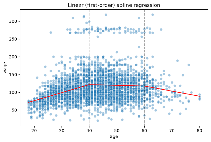
The model plot shows that we have gone from fitting an intercept (i.e., a horizontal line) in each bin to fitting a linear function in each bin.