As we mentioned many times before, it is important to always look at your data! So before we begin with the analysis, lets get a better understanding of the data. For convenience, we create a smaller subset of the main DataFrame:
Additional information: When creating new DataFrames derived from others, they are by default a view or a shallow copy of the original DataFrame. This is due to Pandas optimizing memory usage and access. However, when a shallow copy is created, the data may not be completely decoupled. Only the structure (index and column information) is copied, but the data itself may still reference the original. Sometimes it can therefore be helpful to make a deep copy, which creates an entirely independent object by using the .copy() method.
import pandas as pd

df = pd.read_csv("data/data.txt", delimiter='\t')
df_small = df[['age', 'subject', 'WMf', 'gff']].copy() # Create a deep copy
Descriptive Analysis
We’ll start by examining the first few rows of our new subset using head() and then apply describe() to get an overview of key statistics, such as the mean and standard deviation.
print(df_small.head())
print(df_small.describe())
age subject WMf gff
0 29 111000 0.707143 0.3750
1 23 111001 0.846429 0.3750
2 24 111002 0.744048 0.3125
3 33 111003 0.857143 0.3125
4 29 111004 0.871429 0.4375
age subject WMf gff
count 255.000000 255.000000 255.000000 255.000000
mean 27.368627 271403.650980 0.819362 0.435049
std 4.890674 304680.774051 0.102989 0.175362
min 18.000000 111000.000000 0.530301 0.000000
25% 23.000000 121112.000000 0.764881 0.312500
50% 28.000000 131220.000000 0.830952 0.437500
75% 31.000000 162811.500000 0.895238 0.562500
max 35.000000 952134.000000 1.000000 0.937500
To further visualize the data, we can use Seaborn’s histplot to examine the frequency distribution of the age variable. This will give us a clearer view of how age is distributed across our sample.
#import libraries
import matplotlib.pyplot as plt
import seaborn as sns

sns.histplot(df_small['age'], bins=10);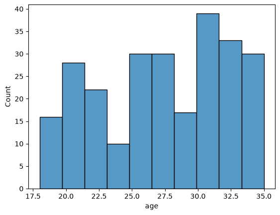
By using Seaborn’s ‘scatterplot’, we can explore the relationship between WMf and gff and identify any trends. Additionally, we will incorporate age as the hue to visualize how this variable may influence the relationship between WMf and gff.
sns.scatterplot(data=df_small, x='WMf', y='gff', hue='age');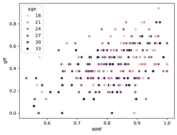
Centering the Predictors
As discussed in the lecture, it is common practice to center predictors in multiple regression around their mean to obtain a meaningful intercept . We can do this by subtracting the mean of each variable from their raw values. We will then save the centered variables to new columns:
df_small['age_c'] = df_small['age'] - df_small['age'].mean()
df_small['WMf_c'] = df_small['WMf'] - df_small['WMf'].mean()

print(df_small.head())
age subject WMf gff age_c WMf_c
0 29 111000 0.707143 0.3750 1.631373 -0.112219
1 23 111001 0.846429 0.3750 -4.368627 0.027066
2 24 111002 0.744048 0.3125 -3.368627 -0.075315
3 33 111003 0.857143 0.3125 5.631373 0.037781
4 29 111004 0.871429 0.4375 1.631373 0.052066
We can now proceed with the actual analysis. To compare multiple linear regression models with centered and non-centered predictors, we can use ols() from Statsmodels and plot the results with the different variables. Let’s create two identical models, one with non-centered predictors, and one with centered ones:
import statsmodels.formula.api as smf

results = smf.ols(formula='gff ~ WMf + age', data=df_small).fit()
print(results.summary())
OLS Regression Results
==============================================================================
Dep. Variable: gff R-squared: 0.240
Model: OLS Adj. R-squared: 0.234
Method: Least Squares F-statistic: 39.75
Date: Wed, 12 Aug 2026 Prob (F-statistic): 9.89e-16
Time: 12:24:01 Log-Likelihood: 117.56
No. Observations: 255 AIC: -229.1
Df Residuals: 252 BIC: -218.5
Df Model: 2
Covariance Type: nonrobust
==============================================================================
coef std err t P>|t| [0.025 0.975]
------------------------------------------------------------------------------
Intercept -0.0268 0.102 -0.263 0.793 -0.228 0.174
WMf 0.7504 0.095 7.927 0.000 0.564 0.937
age -0.0056 0.002 -2.804 0.005 -0.010 -0.002
==============================================================================
Omnibus: 3.651 Durbin-Watson: 1.955
Prob(Omnibus): 0.161 Jarque-Bera (JB): 3.653
Skew: -0.290 Prob(JB): 0.161
Kurtosis: 2.920 Cond. No. 387.
==============================================================================
Notes:
[1] Standard Errors assume that the covariance matrix of the errors is correctly specified.
results = smf.ols(formula='gff ~ WMf_c + age_c', data=df_small).fit()
print(results.summary())
OLS Regression Results
==============================================================================
Dep. Variable: gff R-squared: 0.240
Model: OLS Adj. R-squared: 0.234
Method: Least Squares F-statistic: 39.75
Date: Wed, 12 Aug 2026 Prob (F-statistic): 9.89e-16
Time: 12:24:02 Log-Likelihood: 117.56
No. Observations: 255 AIC: -229.1
Df Residuals: 252 BIC: -218.5
Df Model: 2
Covariance Type: nonrobust
==============================================================================
coef std err t P>|t| [0.025 0.975]
------------------------------------------------------------------------------
Intercept 0.4350 0.010 45.258 0.000 0.416 0.454
WMf_c 0.7504 0.095 7.927 0.000 0.564 0.937
age_c -0.0056 0.002 -2.804 0.005 -0.010 -0.002
==============================================================================
Omnibus: 3.651 Durbin-Watson: 1.955
Prob(Omnibus): 0.161 Jarque-Bera (JB): 3.653
Skew: -0.290 Prob(JB): 0.161
Kurtosis: 2.920 Cond. No. 48.1
==============================================================================
Notes:
[1] Standard Errors assume that the covariance matrix of the errors is correctly specified.
What’s the difference?
In the centered model, the intercept can now be interpreted as the expected fluid intelligence at
the average level of figural working memory
the average age of the range considered in the study.
Centering has no influence on the regression slope coefficients (for
WMfandage).Centering has no influence on the explained variance .