9.2 Moderated Regression - Multivariate Statistics with Python

Moderated regression models are used to understand whether and how the relationship between two variables (a predictor $X_1$ and an outcome $Y$ ) changes at different levels of a third variable (the moderator $X_2$ ). This is accomplished by including an interaction term $(X_1*X_2)$ in the regression model:

Y= b_0+b_1*X_1+b_2*X_2+b_3*(X_1*X_2)

(1)

$Y$ is the predicted value of the dependent variable.
$b_0$ is the intercept.
$b_1$ is the coefficient for the independent variable $X_1$ .
$b_2$ is the coefficient for the moderating variable $X_2$ .
$b_3$ is the coefficient for the interaction term (product of $X_1$ and $X_2$ ).
$(X_1*X_2)$ is the interaction term.

Moderator Variable¶

A moderator variable is a type of independent variable that influences the strength and/or direction of the relationship between another independent variable $X_1$ and a dependent variable $Y$ . In other words, it “moderates” the relationship between the predictor and the outcome. This means that the effect of $X_1$ on $Y$ is not constant but varies depending on the level or value of $X_2$ .

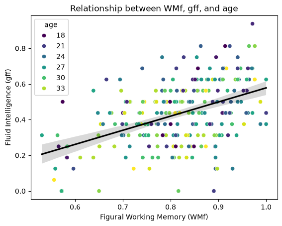
Research question: We investigate whether the association between fluid intelligence (gff) and figural working memory (WMf) is moderated by age (age).

As previously, we can use statsmodels to do so. The regression formula for moderated regression can be specified as y ~ A * B or as y ~ A + B + A:B. A and B are the main effects, A:B is the interaction effect. The first formula is internally automatically expanded to the second one (so if you just want to model the second interaction term you can simply use A:B in a standalone fashion). We will further utilize our centered dataset to obtain a meaningful intercept $b_0$ .

import pandas as pd
import statsmodels.formula.api as smf
import matplotlib.pyplot as plt
import seaborn as sns

df = pd.read_csv("data/data.txt", delimiter='\t')
df_small = df[['age', 'subject', 'WMf', 'gff']].copy() # Create a deep copy

# Center the predictors
df_small['age_c'] = df_small['age'] - df_small['age'].mean()
df_small['WMf_c'] = df_small['WMf'] - df_small['WMf'].mean()

# Fit the model
model = smf.ols(formula='gff ~ WMf_c * age_c', data=df_small)
results = model.fit()
print(results.summary())

                            OLS Regression Results                            
==============================================================================
Dep. Variable:                    gff   R-squared:                       0.243
Model:                            OLS   Adj. R-squared:                  0.233
Method:                 Least Squares   F-statistic:                     26.79
Date:                Wed, 12 Aug 2026   Prob (F-statistic):           4.59e-15
Time:                        12:24:02   Log-Likelihood:                 118.02
No. Observations:                 255   AIC:                            -228.0
Df Residuals:                     251   BIC:                            -213.9
Df Model:                           3                                         
Covariance Type:            nonrobust                                         
===============================================================================
                  coef    std err          t      P>|t|      [0.025      0.975]
-------------------------------------------------------------------------------
Intercept       0.4365      0.010     44.861      0.000       0.417       0.456
WMf_c           0.7489      0.095      7.908      0.000       0.562       0.935
age_c          -0.0055      0.002     -2.754      0.006      -0.009      -0.002
WMf_c:age_c     0.0181      0.019      0.945      0.345      -0.020       0.056
==============================================================================
Omnibus:                        3.536   Durbin-Watson:                   1.947
Prob(Omnibus):                  0.171   Jarque-Bera (JB):                3.557
Skew:                          -0.285   Prob(JB):                        0.169
Kurtosis:                       2.901   Cond. No.                         48.1
==============================================================================

Notes:
[1] Standard Errors assume that the covariance matrix of the errors is correctly specified.

Interpreting the outputs¶

Model overview

Dependent Variable (gff): This is the outcome variable (fluid intelligence) being modeled.
Independent Variables:
- WMf_c: Centered working memory predictor.
- age_c: Centered age predictor.
- WMf_c:age_c: Interaction term between WMf_c and age_c to test for moderation.
R-squared (0.243): Approximately 24.3% of the variance in gff is explained by the predictors in this model.
Adjusted R-squared (0.233): The model explains 23.3% of the variance in gff after accounting for model complexity.

Key Metrics

F-statistic (26.79, p < 0.001): The model as a whole is statistically significant, meaning the predictors collectively explain a significant amount of variance in gff.
Log-Likelihood (118.02): Indicates the model’s goodness-of-fit; higher values suggest better fit.
AIC/BIC (-228.0 / -213.9): Measures of model quality, penalizing complexity. Lower values indicate a better model.

Coefficients

Intercept (0.4365, p < 0.001):
- The expected value of gff when both WMf_c and age_c are at their mean (since these variables are centered).
- This is highly significant, as expected in most models.
WMf_c (0.7489, p < 0.001):
- A positive, significant effect.
- For every unit increase in centered working memory (WMf_c), gff increases by approximately 0.75 units, holding age_c constant.
age_c (-0.0055, p = 0.006):
- A negative, significant effect.
- For every unit increase in centered age (age_c), gff decreases by 0.0055 units, holding WMf_c constant.
Interaction Term WMf_c:age_c (0.0181, p = 0.345):
- This term is not significant (p = 0.345), suggesting no evidence that the relationship between WMf_c and gff changes significantly as a function of age_c.
- In other words, age does not moderate the relationship between working memory and fluid intelligence in this sample.

Summary of findings

Main Effects:
- WMf_c: A strong, positive predictor of gff (fluid intelligence). Higher working memory scores are associated with higher fluid intelligence.
- age_c: A small, negative predictor of gff. Older age is associated with slightly lower fluid intelligence.
Interaction:
- The interaction term (WMf_c:age_c) is not statistically significant, indicating that the effect of working memory on fluid intelligence does not vary significantly across different ages.
Model Fit:
- The model explains a modest proportion of the variance in gff (24.3%), and the predictors collectively contribute significantly.

The regression equation can be written as:

\text{gff}=0.44+0.75 \cdot \text{WMf\_c}-0.0055 \cdot \text{age\_c}+0.018 \cdot \text{WMf\_c} \cdot \text{age\_c}

(2)

The following plot illustrates the relationship between WMf, gff and age as their moderator (please note that the regression line is only a simple linear regression!).

import matplotlib as mpl

fig, ax = plt.subplots()
sns.scatterplot(data=df_small, x='WMf', y='gff', hue='age', palette='viridis', ax=ax)
sns.regplot(data=df_small, x='WMf', y='gff', scatter=False, color='black', ax=ax)
ax.set(xlabel='Figural Working Memory (WMf)', ylabel='Fluid Intelligence (gff)', title='Relationship between WMf, gff, and age')

plt.show()