In neurocognitive psychology, we often collect huge amounts of data. Sometimes we can have thousands of measurements from different brain regions or many behavioral scores. Having more information can, in theory, help us make better predictions, but it also brings risks: too many variables can make analyses infeasible, lead to false discoveries, or cause models to learn noise instead of real effects.
The large p issue
Big data refers to large data sets with many predictors which often cannot be processed or analyzed using traditional data processing techniques. For our prediction models, this brings some issues:
While the linear model can in theory still be used for such data, the ordinary least squares fit becomes infeasible, especially when p > n
The large amount of features reduce interpretability
This is where linear model selection becomes essential, offering techniques to refine our models and extract meaningful insights from high-dimensional data.
Today’s data: Hitters
For practical demonstration, we will use the Hitters dataset. This dataset provides Major League Baseball Data from the 1986 and 1987 seasons. It contains 322 observations of major league players on 20 variables (so it’s not big data, but we can pretend it is). The Research aim is to predict a baseball player’s salary on the basis of various predictors associated with the performance in the previous year. You can check its contents here: https://
import statsmodels.api as sm

# Get the data
hitters = sm.datasets.get_rdataset("Hitters", "ISLR").data
For computational reasons, we will not include all predictors but only a smaller subset:
# Keep a total of 10 variables - the target ´Salary´ and 9  features.
hitters_subset = hitters[["Salary", "CHits", "CAtBat", "CRuns", "CWalks", "Assists", "Hits", "HmRun", "Years", "Errors"]].copy()

# Remove rows with missing values
hitters_subset.dropna(inplace=True)

hitters_subset.head()Let’s also take a look at the correlation matrix to check for potential multicollinearity, which can affect the stability of linear regression models.
import seaborn as sns

sns.heatmap(hitters_subset.corr(), annot=True, cmap="coolwarm", fmt=".2f");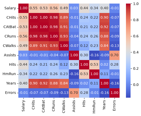
The heatmap reveals strong correlations between several predictors:
CHitsandCAtBatcorrelate at 0.995 (displayed as 1.00 after rounding)CHitsandCRunscorrelate at 0.985
We thus remove two of the correlated features:
features_drop = ["CRuns", "CAtBat"]
hitters_subset = hitters_subset.drop(columns=features_drop)
Handling big data in linear models
Subset Selection
In subset selection we identify a subset of the predictors that are truly related to the outcome. The model is then fitted using least squares on the reduced set of variables.
How do we determine which variables are relevant?
Best Subset Selection
We will start with performing Best Subset Selection (also called exhaustive search) as implemented in the mlxtend package. It has great documentation, e.g. for the exhaustive search. In short, this approach is a brute-force evaluation of feature subsets. A specific performance metric (e.g. MSE, R², or accuracy) is optimized given an arbitrary regressor or classifier. For example, if we have 4 features, the algorithm will evaluate all 15 possible combinations of features.
Before we start the subset selection, we first define the target and the features:
import numpy as np

y = hitters_subset["Salary"]
X = hitters_subset.drop("Salary", axis=1)
We first split our data into training and test dataset. Although the selection function uses cross-validation to identify the best subset of predictors (Step 3), this evaluation is done during the selection process and can still overfit to the data. To fairly assess how the final model performs on new data, we split off a test set and use it only after feature selection is complete.
from sklearn.model_selection import train_test_split

X_train, X_test, y_train, y_test = train_test_split(X, y, test_size=0.3, random_state=42)| Purpose | What is it for? | When? |
|---|---|---|
| Cross Validation in selection function | Helps choose the best subset of features | During selection |
| Test Set Evaluation | Checks how well the final model performs | After selection |
We then run Best Subset Selection on the training data:
from sklearn.linear_model import LinearRegression
from mlxtend.feature_selection import ExhaustiveFeatureSelector

efs = ExhaustiveFeatureSelector(
        estimator=LinearRegression(),
        min_features=1,
        max_features=X_train.shape[1],
        scoring='r2',
        cv=5,
        print_progress=False)

efs.fit(X_train, y_train)

print('Best R²: %.2f' % efs.best_score_)
print('Best subset (indices):', efs.best_idx_)
print('Best subset (corresponding names):', efs.best_feature_names_)
Best R²: 0.41
Best subset (indices): (1, 3, 4)
Best subset (corresponding names): ('CWalks', 'Hits', 'HmRun')
If you are interested in the details, they are stored in the metric dictionary:
import pandas as pd

df = pd.DataFrame.from_dict(efs.get_metric_dict()).T
df.sort_values('avg_score', inplace=True, ascending=False)
dfForward Stepwise Selection
Forward Stepwise Selection is a greedy feature‐selection method that starts with no features and, at each step, adds the single feature whose inclusion most improves the model’s performance. This “add the best remaining feature” is repeated until a desired number of features is reached, at which point the algorithm stops and returns the best subset.
An important parameter is k_features, which determines the number of features to select. We can, pass an integer (must be less than the total number of available features), a tuple (the algorithm will then evaluate all subset sizes between the min and max value), or one of two string options ("best", or "parsimonious"). Please refer to the documentation for further details.
from mlxtend.feature_selection import SequentialFeatureSelector

sfs_forward = SequentialFeatureSelector(
    estimator=LinearRegression(),
    k_features=(1, X_train.shape[1]),
    forward=True,
    scoring='r2',
    cv=5,
    verbose=0)

sfs_forward.fit(X_train, y_train)

print(f">> Forward SFS:")
print(f"   Best CV R²      : {sfs_forward.k_score_:.3f}")
print(f"   Optimal # feats : {len(sfs_forward.k_feature_idx_)}")
print(f"   Feature indices : {sfs_forward.k_feature_idx_}")
print(f"   Feature names   : {sfs_forward.k_feature_names_}")
>> Forward SFS:
Best CV R² : 0.413
Optimal # feats : 3
Feature indices : (1, 3, 4)
Feature names : ('CWalks', 'Hits', 'HmRun')
You can see we ended up with the same three predictors as in best subset selection: CWalks, Hits, HmRun. However, this is not necessarily always the cas! Best subset and stepwise selection can, and often do, lead to different results. In our case we only had a small number of predictors, which makes it more likely to end up with the same subset.
Backward Stepwise Selection
Backward Stepwise Selection begins with the full feature set and, at each step, removes the single feature whose exclusion most improves (or least harms) model performance. We keep repeating this “remove the worst feature” step until only the desired number of features remains, and then the algorithm returns that reduced subset:
sfs_backward = SequentialFeatureSelector(
    estimator=LinearRegression(),
    k_features=(1, X_train.shape[1]),
    forward=False,
    floating=False,
    scoring='r2',
    cv=5,
    verbose=0)

sfs_backward.fit(X_train, y_train)

print(f"<< Backward SFS:")
print(f"   Best CV R²      : {sfs_backward.k_score_:.3f}")
print(f"   Optimal # feats : {len(sfs_backward.k_feature_idx_)}")
print(f"   Feature indices : {sfs_backward.k_feature_idx_}")
print(f"   Feature names   : {sfs_backward.k_feature_names_}")
<< Backward SFS:
Best CV R² : 0.413
Optimal # feats : 3
Feature indices : (1, 3, 4)
Feature names : ('CWalks', 'Hits', 'HmRun')
Scikit-learn Alternative
Scikit-learn provides SequentialFeatureSelector
as an alternative to mlxtend’s stepwise selection. It supports both forward and backward selection via the direction parameter:
from sklearn.feature_selection import SequentialFeatureSelector

sfs_sklearn = SequentialFeatureSelector(
    estimator=LinearRegression(),
    n_features_to_select="auto",
    direction="forward",
    scoring="r2",
    cv=5)

sfs_sklearn.fit(X_train, y_train)

print(f"   Selected features: {X_train.columns[sfs_sklearn.get_support()].tolist()}")
Selected features: ['CWalks', 'Hits', 'HmRun']
Note that you can here either specify n_features_to_select directly, or you can use "auto" with a tol parameter that stops adding features once the score improvement falls below the threshold.
Summary
| Selection Method | Finds best model? | Works for large p? | Works for p>n? | Computational cost |
|---|---|---|---|---|
| Best Subset | + Yes | - No | - No | - Very high |
| Forward Stepwise | - No | + Moderate/large p | o If model size < n | + Efficient |
| Backward Stepwise | - No | + Yes (only if p < n) | - No | o Relatively Efficient |
What next?
All three procedures converged on the same three predictors here, so let’s evaluate the model performance and estimate the true test error using that subset.
import numpy as np
from sklearn.metrics import mean_squared_error, r2_score
from sklearn.linear_model import LinearRegression

selected_features = list(sfs_forward.k_feature_names_)

# Subset the data
X_train_subset = X_train[selected_features]
X_test_subset = X_test[selected_features]

# Fit the model
model = LinearRegression()
model.fit(X_train_subset, y_train)

# Get predictions and performance
y_pred = model.predict(X_test_subset)

mse_test = mean_squared_error(y_test, y_pred)
rmse_test = np.sqrt(mse_test)
r2_test = r2_score(y_test, y_pred)

print(f"Test MSE:  {mse_test:.2f}")
print(f"Test RMSE: {rmse_test:.2f}")
print(f"Test R²:   {r2_test:.4f}")
Test MSE: 182321.00
Test RMSE: 426.99
Test R²: 0.2492
So in sum:
On average, our predictions deviate from the actual salary by about 426 thousand dollars.
Our model explains ~25% of the variance in salary.
Regularization and Dimensionality Reduction
As mentioned before, regularization and dimensionality reduction are two other measures of dealing with large numbers of predictors. Regularization techniques will be introduced in the next session, and dimensionality reduction will be introduced in the Principal Component Analysis session.