🌳 Decision Trees - Statistical Learning with Python

Decision Trees are powerful and intuitive models used for both classification and regression problems. They work by recursively partitioning the feature space into smaller regions and assigning a prediction to each one. The tree structure is easy to interpret and visualise, making it a popular choice for understanding the relationship between inputs and outputs.

At their core, decision trees split the dataset into subsets based on feature values. Each split is chosen to minimise an impurity measure (equivalently, to maximise the information we gain about the target), with the goal of producing child nodes that are as homogeneous as possible.

Some key terminology:

Nodes: Every point in the tree. Either an internal node, where a split happens, or a leaf node, where a prediction is assigned.
Leaves (terminal nodes): Regions of the feature space with a predicted outcome.
Splits: Binary decisions on feature values, e.g., “is BMI ≤ 25?”. This is where two new branches are created.

Fitting a tree uses an algorithm called recursive binary splitting:

Binary: each split produces two branches. “Yes” or “no” on a single condition.
Recursive: the same procedure is then applied to each child, until a stopping criterion is reached (e.g. minimum node size, maximum depth).
Greedy & top-down: starting from the root, each node picks the split that looks best right now (largest impurity reduction), without looking ahead. This is fast and practical, but not guaranteed to be globally optimal.

Splitting Criteria: What Makes a Good Split?¶

Every internal node faces the same question: which feature, and at which threshold, should we split on? A split is “good” if the resulting children are more homogeneous than the parent. To make this precise we need an impurity measure. Classification and regression use different ones.

Classification: Gini and Entropy¶

For a node containing samples from $K$ classes, let $p_k$ be the proportion of samples in class $k$ . The two most common impurity measures are:

Gini impurity

G = 1 - \sum_{k=1}^{K} p_k^2

(1)

Gini can be read as the probability of misclassifying a randomly drawn sample from the node if we predicted its class at random according to the node’s class proportions. It is 0 when the node is pure (one class only) and reaches its maximum when classes are evenly mixed (0.5 for two classes, $1 - 1/K$ in general).

Entropy

H = -\sum_{k=1}^{K} p_k \log_2 p_k

(2)

Entropy comes from information theory and measures the average “surprise” of the labels in the node. Like Gini, it is 0 for a pure node and maximal for a perfectly balanced mix (1 bit for two classes).

In practice, Gini and entropy almost always select similar splits. Gini is the scikit-learn default, mainly because it avoids the logarithm and is a little bit faster to compute.

Information Gain: Comparing Candidate Splits¶

Once we have an impurity measure $I$ , the quality of a candidate split is the reduction in impurity from parent to children, weighted by the size of each child:

\text{Gain} = I(\text{parent}) - \sum_{c \in \{\text{left, right}\}} \frac{N_c}{N}\, I(c)

(3)

The algorithm tries every feature and every possible threshold, picks the split with the largest gain, and recurses. This is greedy, which means it only looks one step ahead, but it works remarkably well in practice.

Worked example

Suppose a node contains 10 samples: 6 from class A and 4 from class B.

Gini at the node: $1 - (0.6^2 + 0.4^2) = 0.48$
Entropy at the node: $-(0.6 \log_2 0.6 + 0.4 \log_2 0.4) \approx 0.971$

Now imagine a candidate split produces:

Left child (6 samples): 5 A, 1 B → $G_\text{left} = 1 - (5/6)^2 - (1/6)^2 \approx 0.278$
Right child (4 samples): 1 A, 3 B → $G_\text{right} = 1 - (1/4)^2 - (3/4)^2 = 0.375$

Weighted child Gini: $\tfrac{6}{10}(0.278) + \tfrac{4}{10}(0.375) \approx 0.317$ .

Information gain (with Gini): $0.48 - 0.317 \approx 0.163$ .

The algorithm computes this for every candidate split and chooses the one with the largest gain.

Regression: Variance Reduction¶

For regression the target is continuous, so impurity is naturally measured by the mean squared error of the response within a node:

I(\text{node}) = \frac{1}{N} \sum_{i \in \text{node}} (y_i - \bar{y})^2

(4)

where $\bar{y}$ is the mean response in the node. Choosing a split that minimises the weighted child MSE is equivalent to maximising the variance reduction. The leaf prediction is simply the mean of the training points that fall into it.

Regression Trees¶

The general usage of regression trees is identical to previous regression models:

from sklearn.tree import DecisionTreeRegressor

model = DecisionTreeRegressor()
model.fit(X_train, y_train)
model.predict(X_test)

As you learned in the lecture, there are a few additional parameters which we can choose, such as stopping criteria (when to stop splitting). You can look these up in the documentation. To see how these models perform, we can simply plot the predictions for two different models on synthetic data.

Generate data:

import numpy as np
from sklearn.model_selection import train_test_split

rng = np.random.RandomState(1)
X = np.sort(5 * rng.rand(100, 1), axis=0)
y = np.sin(X).ravel()
y[::5] += 3 * (0.5 - rng.rand(20))

X_train, X_test, y_train, y_test = train_test_split(X, y, test_size=0.3, random_state=0)

Fit two decision tree regressors to the data

from sklearn.tree import DecisionTreeRegressor

model1 = DecisionTreeRegressor(max_depth=2)
model2 = DecisionTreeRegressor(max_depth=6)

model1.fit(X_train, y_train)
model2.fit(X_train, y_train);

Plot the predictions to see how different models behave:

import matplotlib.pyplot as plt

X_range = np.arange(0.0, 5.0, 0.01)[:, np.newaxis]
pred1 = model1.predict(X_range)
pred2 = model2.predict(X_range);

plt.figure()
plt.scatter(X, y, s=30, c="darkorange", label="data")
plt.plot(X_range, pred1, color="cornflowerblue", label="max_depth=2", linewidth=2)
plt.plot(X_range, pred2, color="yellowgreen", label="max_depth=6", linewidth=2)
plt.xlabel("data")
plt.ylabel("target")
plt.title("Decision Tree Regression")
plt.legend();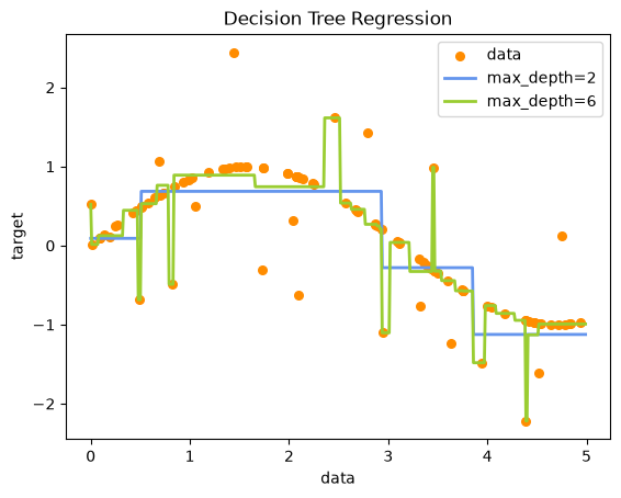

You can see that the max_depth=2 model is underfitting, while the max_depth=6 is overfitting. We can also evaluate the models with usual performance metrics such as $R^2$ :

from sklearn.metrics import r2_score

r2_1 = r2_score(y_test, model1.predict(X_test))
r2_2 = r2_score(y_test, model2.predict(X_test))

print(f"R² (max_depth=2): {r2_1:.3f}")
print(f"R² (max_depth=6): {r2_2:.3f}")

R² (max_depth=2): 0.571
R² (max_depth=6): 0.472

Classification Trees¶

The general usage of classification trees is identical to previous classification models:

import matplotlib.pyplot as plt
from sklearn.tree import DecisionTreeClassifier, plot_tree
from sklearn.datasets import load_iris

# Load data
iris = load_iris()
X, y = iris.data, iris.target

clf = DecisionTreeClassifier(max_depth=3)
clf.fit(X, y)

plt.figure(figsize=(12,8))
plot_tree(clf, feature_names=iris.feature_names, class_names=iris.target_names, filled=True, rounded=True, fontsize=14);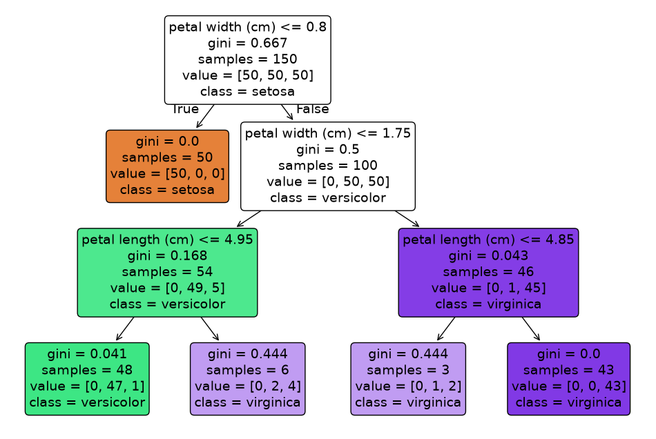

The tree plot of the fitted model contains the following information:

Decision nodes
- These are the rectangles with a splitting criterion (e.g. feature ≤ threshold)
- They represent the points where the model splits the data and asks “which branch next?”
Edges
- The lines connecting nodes
- Left edge follows the true branch (node condition met), right edge the false branch
Leaf nodes
- The terminal rectangles without further splits
- The leaf nodes mark the final predicted class (class)
Color fill
- The hue corresponds to the majority class at that node
- The depth of color indicates purity (dark = almost all one class; light = mixture)
Gini or entropy (shown as the first line of each node)
- Quantifies how “mixed” a node is and drives the choice of split
- Pure nodes (all same class) are darkest with the colour of that class; perfectly mixed nodes are white
Tree depth
- The number of levels indicates how many successive decisions are made
- Capped by the max_depth parameter to control complexity

Another nice illustration is plotting the decision boundaries. As this works mostly with 2 features, we plot pairwise feature combinations:

import numpy as np
from sklearn.inspection import DecisionBoundaryDisplay

# Plot settings
pairs      = [(0,1), (0,2), (0,3), (1,2), (1,3), (2,3)]
n_classes  = len(iris.target_names)
colors     = ["r", "g", "b"]
fig, axes  = plt.subplots(2, 3, figsize=(12, 8))
axes       = axes.ravel()

for ax, (i, j) in zip(axes, pairs):
    X_sub = X[:, [i, j]]
    clf = DecisionTreeClassifier(max_depth=4)
    clf.fit(X_sub, y)

    # Plot decision surface
    disp = DecisionBoundaryDisplay.from_estimator(
              clf, X_sub, cmap=plt.cm.RdYlBu, response_method="predict", 
              ax=ax, xlabel=iris.feature_names[i], ylabel=iris.feature_names[j])

    # Overlay training points
    for class_idx, color in zip(range(n_classes), colors):
        mask = (y == class_idx)
        ax.scatter(X_sub[mask, 0], X_sub[mask, 1], c=color, label=iris.target_names[class_idx], edgecolor="k", s=25)

    ax.set_title(f"{iris.feature_names[i]} vs {iris.feature_names[j]}")

# Legend and layout
handles, labels = axes[0].get_legend_handles_labels()
fig.legend(handles, labels, loc="lower center", ncol=n_classes, frameon=False)
fig.suptitle("Decision Surfaces")
plt.tight_layout();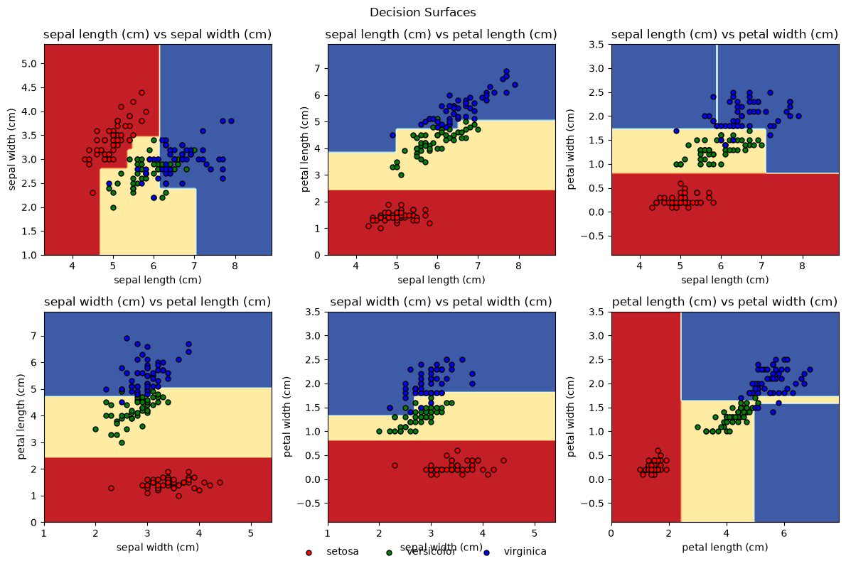

Overfitting¶

Large trees tend to overfit. To counter this we can do multiple things:

Prune the full-grown tree (post-pruning), also called cost-complexity pruning (we saw this in the lecture)
Tune the hyperparameters that control the tree-growing behaviour (pre-pruning)
Ensemble methods: bagging, random forests and boosting (will be introduced later)

Cost Complexity Pruning & Hyperparameter Tuning¶

Cost complexity pruning means we add a penalty for tree size:

$\text{Total Cost} = \text{RSS or Classification Error} + \alpha \cdot \text{Tree Size}$

In scikit-learn this is controlled by ccp_alpha

ccp_alpha = 0 -> no pruning -> full-grown tree
ccp_alpha > 0 -> pruning -> smaller tree

Scikit-learn can return the sequence of $\alpha$ values at which one or more branches get pruned via cost_complexity_pruning_path. We can then refit the tree at each $\alpha$ and watch how train and test accuracy change as the tree gets progressively simpler:

from sklearn.model_selection import train_test_split

iris = load_iris()
X, y = iris.data, iris.target
X_train, X_test, y_train, y_test = train_test_split(X, y, test_size=0.3, random_state=0)

# Sequence of effective alphas along the pruning path
path = DecisionTreeClassifier(random_state=0).cost_complexity_pruning_path(X_train, y_train)
alphas = path.ccp_alphas[:-1]  # drop the trivial single-node tree at the end

train_scores, test_scores = [], []
for a in alphas:
    clf = DecisionTreeClassifier(ccp_alpha=a, random_state=0).fit(X_train, y_train)
    train_scores.append(clf.score(X_train, y_train))
    test_scores.append(clf.score(X_test, y_test))

plt.figure()
plt.plot(alphas, train_scores, marker='o', label='Train')
plt.plot(alphas, test_scores,  marker='o', label='Test')
plt.xlabel(r'$\alpha$ (ccp_alpha)')
plt.ylabel('Accuracy')
plt.title('Cost-complexity pruning path')
plt.legend();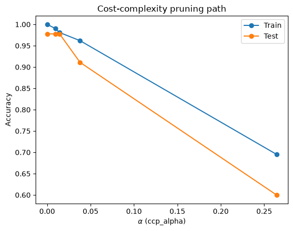

At $\alpha = 0$ the tree fits the training set almost perfectly but generalises less well. As $\alpha$ grows, the tree gets smaller: training accuracy drops, but test accuracy often improves in a sweet-spot region before the tree becomes too simple to capture the signal.

Pre-pruning via Hyperparameters¶

The same goal of avoiding over-grown trees can be approached by limiting how the tree is allowed to grow in the first place — this is what pre-pruning does, in contrast to the post-pruning performed by ccp_alpha:

max_depth: maximum depth of the tree
min_samples_split: minimum number of samples required to split an internal node
min_samples_leaf: minimum number of samples that must end up in a leaf

A grid search lets us find a good combination of these (and ccp_alpha) at the same time:

from sklearn.model_selection import GridSearchCV

param_grid = {
    'ccp_alpha':         np.linspace(0.0, 0.05, 6),
    'max_depth':         [2, 4, 6, 8, None],
    'min_samples_split': [2, 5, 10],
    'min_samples_leaf':  [1, 2, 4],
}

grid = GridSearchCV(DecisionTreeClassifier(random_state=0), param_grid, cv=5)
grid.fit(X_train, y_train)

print("Best params:", grid.best_params_)
print("Test set accuracy:", grid.score(X_test, y_test))

Best params: {'ccp_alpha': np.float64(0.0), 'max_depth': 4, 'min_samples_leaf': 1, 'min_samples_split': 5}
Test set accuracy: 0.9777777777777777

Ensemble Methods¶

Single trees have high variance: a small change in the training data can lead to a very different tree. They also tend to overfit and are often not competitive with other strong models like support vector machines. Ensemble methods address these issues by combining many trees, primarily to reduce variance (bagging, random forest) or bias (boosting).

Bagging (Bootstrap Aggregation)¶

Bagging involves the following steps:

Create multiple bootstrapped samples of the training set (i.e. samples drawn with replacement, each of the same size as the original).
Train one tree (typically grown deep, without pruning) on each sample.
Aggregate the predictions across all trees:
- Classification: majority vote
- Regression: average prediction

Why does this work? Deep trees have low bias but high variance. This means they fit complex patterns but are very sensitive to the particular training sample. Averaging many such predictors leaves the bias unchanged but reduces the variance, provided the individual predictors are not too correlated. Bootstrapping is what introduces enough variation between trees for the averaging to actually help.

from sklearn.ensemble import BaggingClassifier
from sklearn.metrics import accuracy_score

bag = BaggingClassifier(n_estimators=100, random_state=0)
bag.fit(X_train, y_train)

accuracy_score(y_test, bag.predict(X_test))

0.9777777777777777

Random Forest¶

A weakness of plain bagging is that, if one feature is very predictive, every tree will tend to split on it first. So the trees will end up highly correlated, and averaging gains less than we’d hope. Random forests still use bagging’s bootstrap samples, but add a second source of randomness: at each split, only a random subset of features is considered as candidates. The defaults are:

$\sqrt{p}$ features per split for classification
$p/3$ features per split for regression

This decorrelates the trees and typically gives a noticeable accuracy bump over plain bagging.

A useful side effect of bootstrapping: about 1/3 of the training samples are not in any given tree’s bootstrap sample. These out-of-bag (OOB) samples can be used to estimate generalisation performance without holding out a separate validation set:

Where does the 1/3 come from?

A bootstrap sample is drawn with replacement, $n$ times from the $n$ training samples. For one specific sample $x_i$ :

Probability it is not picked on a single draw: $\left(1 - \tfrac{1}{n}\right)$
Probability it is not picked on any of the $n$ draws: $\left(1 - \tfrac{1}{n}\right)^n$

As $n$ grows this converges to a classic limit:

\lim_{n \to \infty}\left(1 - \tfrac{1}{n}\right)^n = \frac{1}{e} \approx 0.368

(5)

So about 36.8% of the training set ends up out-of-bag for any given tree. Even at modest $n$ we are already near the limit (e.g. $n = 50$ gives ≈ 0.364).

from sklearn.ensemble import RandomForestClassifier

rf = RandomForestClassifier(n_estimators=100, oob_score=True, random_state=0)
rf.fit(X_train, y_train)

print(f"OOB score:     {rf.oob_score_:.3f}")
print(f"Test accuracy: {accuracy_score(y_test, rf.predict(X_test)):.3f}")

OOB score:     0.952
Test accuracy: 0.978

Random forests also give us feature importances: a measure of how much each feature reduces impurity (averaged across all splits and all trees in which it appears).

import seaborn as sns

sns.barplot(x=rf.feature_importances_, y=iris.feature_names)
plt.title("Feature Importance");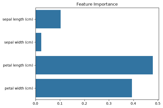

Boosting¶

Where bagging trains trees in parallel on bootstrap samples, boosting trains them sequentially: each new tree tries to fix the mistakes of the ensemble so far. The two most common flavours are:

AdaBoost: after each round, training samples that were misclassified get a higher weight, so the next tree focuses on the hardest cases. Final predictions are a weighted vote.
Gradient Boosting: each new tree is fit to the gradient of the loss function with respect to the current predictions. For squared-error loss this gradient means we are simply fitting the residuals $y - \hat{y}$ .

Because boosting actively reduces both bias and variance, it tends to be the strongest off-the-shelf method on tabular data, but it is more sensitive to hyperparameters than bagging. The main knobs are:

n_estimators: number of trees (more = lower bias but slower and risk of overfitting)
learning_rate ( $\eta$ ): shrinks each tree’s contribution; smaller values need more trees but generalise better
max_depth: depth of each individual tree (boosting traditionally uses shallow trees, often depth 3–6)

Scikit-learn provides GradientBoostingClassifier for the classical implementation, plus HistGradientBoostingClassifier for a faster histogram-based variant. Outside scikit-learn, the most popular implementations are XGBoost, LightGBM, and CatBoost, which typically scale better to very large datasets.

from sklearn.ensemble import GradientBoostingClassifier

boost = GradientBoostingClassifier(n_estimators=100, learning_rate=0.1, max_depth=3, random_state=0)
boost.fit(X_train, y_train)
accuracy_score(y_test, boost.predict(X_test))

0.9777777777777777

Putting It All Together¶

To wrap up (and have all the implementations in a single place), let’s compare all four approaches on the same Iris split. Because Iris is tiny and easy, they all give the same result:

import pandas as pd

models = {
    "Single tree":   DecisionTreeClassifier(max_depth=3, random_state=0),
    "Bagging":       BaggingClassifier(n_estimators=100, random_state=0),
    "Random forest": RandomForestClassifier(n_estimators=100, random_state=0),
    "Boosting":      GradientBoostingClassifier(n_estimators=100, learning_rate=0.1, max_depth=3, random_state=0),
}

results = []
for name, model in models.items():
    model.fit(X_train, y_train)
    results.append((name, accuracy_score(y_test, model.predict(X_test))))

pd.DataFrame(results, columns=["Model", "Test accuracy"])

Summary¶

Summary

Method	Description	Pros	Cons
Decision Trees	Split data via feature thresholds	Highly interpretable, fast to train	High variance → prone to overfitting
Bagging	Average many bootstrapped trees	Reduces variance / overfitting	Less interpretable; larger memory footprint
Random Forest	Bagging + random feature subsets at each split	Further reduces variance; robust	Slower to train and predict
Boosting	Sequentially fit to previous residuals / errors	Low bias → often very accurate	Can overfit noisy data; sensitive to hyperparameters