Building on subset selection, an alternative approach is to include all p predictors in the model but apply regularization—shrinking the coefficient estimates toward zero relative to the least squares estimates. This reduces model complexity without fully discarding variables. Though it introduces some bias, it often lowers variance and improves test performance.
3 approaches are commonly used to regularize the predictors:
Ridge Regression (L2 Regression)
Lasso Regression (L1 Regression)
Elastic Net Regression
Today’s data: Hitters
For practical demonstration, we will again use the Hitters dataset.
import statsmodels.api as sm

hitters = sm.datasets.get_rdataset("Hitters", "ISLR").data

# Keep 15 variables - the target ´Salary´ and 14 features.
hitters_subset = hitters[["Salary", "AtBat", "Runs","RBI", "CHits", "CAtBat", "CRuns", "CWalks", "Assists", "Hits", "HmRun", "Years", "Errors", "Walks"]].copy()
hitters_subset = hitters_subset.drop(columns=["CRuns", "CAtBat"]) # Remove highly correlated features (see previous session)
hitters_subset.dropna(inplace=True) # drop rows containing missing data

hitters_subset.head()Once again, let’s take a look at the correlation between predictors to check for potential multicollinearity, which can affect the stability of linear regression models:
import seaborn as sns

sns.heatmap(hitters_subset.corr(), annot=True, cmap="coolwarm", fmt=".2f");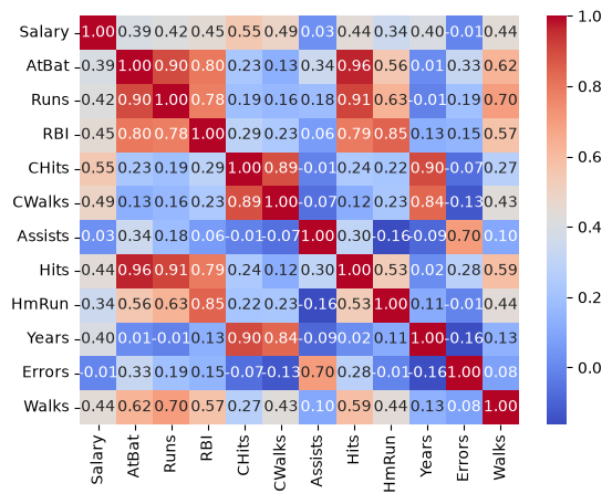
We now continue to prepare our data by defining target and features and split it into training and test set:
from sklearn.model_selection import train_test_split

y = hitters_subset["Salary"]
X = hitters_subset.drop(columns=["Salary"])

X_train, X_test, y_train, y_test = train_test_split(X, y, test_size=0.3, random_state=42)
Great! We are now ready for using the data in our regression models.
Ridge Regression
The loss function for ridge regression is defined as:
Where:
is the number of observations
is the number of predictors
is the target for observation is the row vector of features for observation
are the regression coefficients
is the regularization strength
Combined:
is the residual sum of squares (RSS)
is the L2 penalty on the coefficients
Implementing Ridge Regression
Step 1: We first standardize the predictors as ridge regression is sensitive to scaling. This can be done by using e.g. StandardScaler from scikit-learn:
from matplotlib import pyplot as plt
from sklearn.preprocessing import StandardScaler

scaler = StandardScaler() # Scale predictors to mean=0 and std=1
X_train_scaled = scaler.fit_transform(X_train)
X_test_scaled = scaler.transform(X_test)
Step 2: Next, we set up a range of values for λ. We will test 100 values between 0.001 and 150:
import numpy as np

lambda_range = np.linspace(0.001, 150, 100)
Step 3: For each lambda, we will perform ridge regression on the training data. Cross-validation is then used to identify the optimal lambda that minimizes prediction error:
from sklearn.linear_model import RidgeCV
import pandas as pd

# Get the optimal lambda
ridge_cv = RidgeCV(alphas=lambda_range, cv=5)
ridge_cv.fit(X_train_scaled, y_train)

print(f"Optimal alpha: {ridge_cv.alpha_}")

# Get training R²
train_score_ridge= ridge_cv.score(X_train_scaled, y_train)
print(f"Training R²: {train_score_ridge}")
Optimal alpha: 96.97005050505051
Training R²: 0.4608165508297104
We can then inspect the coefficients of the regression model:
# Put the coefficients into a nicely formatted df for visualization
coef_table = pd.DataFrame({
    'Predictor': X_train.columns,
    'Beta': ridge_cv.coef_
})

coef_table = coef_table.reindex(coef_table['Beta'].abs().sort_values(ascending=False).index)
print(coef_table)
Predictor Beta
3 CHits 76.228175
6 Hits 56.968470
4 CWalks 48.304183
8 Years 41.872502
1 Runs 32.312795
7 HmRun 30.460475
2 RBI 29.460997
10 Walks 29.326931
0 AtBat 22.572136
9 Errors -7.159927
5 Assists -7.051631
Step 4: Finally, we can evaluate the model on the testing data to assess its ability for generalization:
test_score_ridge = ridge_cv.score(X_test_scaled, y_test)

print(f"Test R²: {test_score_ridge}")
Test R²: 0.2919361632717047
Additional visualization: To get a better intuition about how different lambda values affect the beta estimates, we can simply plot them for each model:
from sklearn.linear_model import Ridge
import numpy as np

coefs = []
alphas = np.linspace(0.001, 50, 100)

for a in alphas:
  ridgereg = Ridge(alpha=a)
  ridgereg.fit(X_train_scaled,y_train)
  coefs.append(ridgereg.coef_)

# Plot
fig, ax = plt.subplots()
ax.plot(alphas, coefs)
ax.set(title="Ridge coefficients", xlabel="Lambda", ylabel="Beta");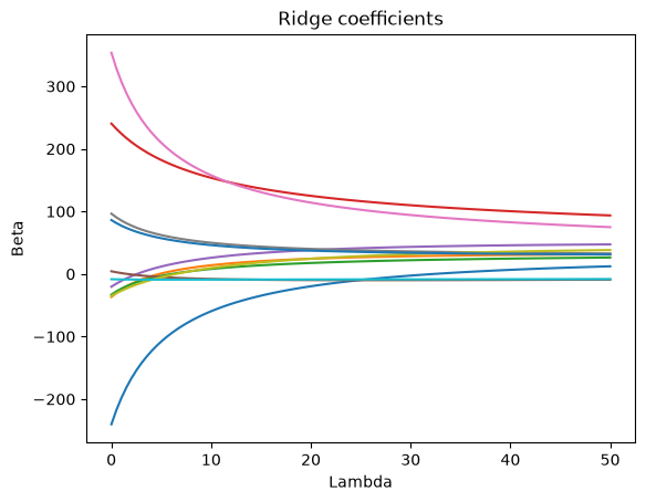
Lasso Regression
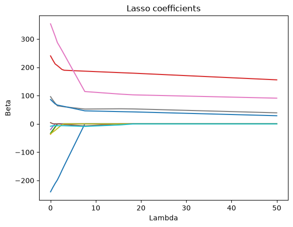
In contrast to ridge regression, lasso regression will not retain all predictors in the final model but force some of them to zero. The loss function for lasso is given as:
Where:
is the residual sum of squares (RSS)
is the L1 penalty on the coefficients
You can see, that the concept is nearly identical, with the only difference being the form of the penalty term. Lasso uses the L1 norm () while Ridge uses the L2 norm (). Because of this geometric difference in the penalty, Lasso can produce sparse models by zeroing out irrelevant features, whereas Ridge keeps all predictors in the model but with smaller weights. Both balance the trade‐off between model fit (the RSS term) and complexity via the tuning parameter λ, typically chosen by cross‐validation.
Why Ridge and Lasso Behave Differently: The Budget
When we use Ridge or Lasso regression, we are not just trying to fit the data perfectly — we are also trying to control how large the coefficients become. If we let them grow without any limits, the model could become too complex and overfit the data.
To prevent this, Ridge and Lasso add a kind of budget: We are only allowed to spend a certain amount on the size of the coefficients. You can think of it like having a fixed amount of money that you have to divide up among all your coefficients.
This budget is enforced by a mathematical condition. For Lasso, the total absolute value of the coefficients must stay below a certain limit :
For Ridge, the total squared value of the coefficients must stay below this limit:
Even though both Ridge and Lasso limit the size of the coefficients, how they limit them is different — and this changes the behaviour of the models.
In Lasso regression (left plot), the constraint forms a diamond shape (or a “pointy” version in higher dimensions). Because of these sharp corners, Lasso often drives some coefficients exactly to zero — which is why Lasso can create sparse models (feature selection).
In Ridge regression (right plot), the constraint forms a circular shape (or a sphere in higher dimensions). This means that Ridge tends to shrink coefficients smoothly but rarely sets them exactly to zero.
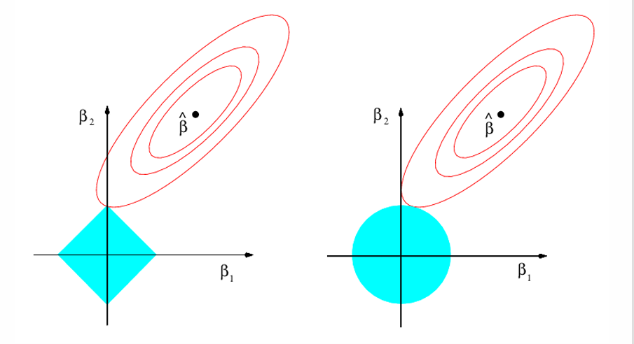
Figure 1:The budget for Lasso and Ridge regression.
Elastic Net Regression
Neither Ridge nor Lasso will universally be better than the other. The main difference between them is the coefficient selection:
Lasso tends to shrink some coefficients all the way to zero, effectively performing feature selection by excluding less relevant variables.
Ridge also shrinks coefficients toward zero, but does not eliminate any completely. Instead of selecting variables, it distributes the effect across all features.
Another point to note is their response to multicollinearity:
Ridge shares the weight among collinear features, keep them all (shrink but don’t zero)
Lasso chooses a subset (often just one) from each collinear group and zero out the rest
This is where elastic net regression comes into play. Elastic net is a combination of Ridge and Lasso:
Here, the mixing parameter determines how much weight to give each penalty: when you recover pure Lasso (only an L1 penalty), and when you recover pure Ridge (only an L2 penalty); values in between blend the two. By combining these penalties, Elastic Net can both shrink coefficients (like Ridge) and select variables (like Lasso), while also tending to select or drop groups of correlated features together. In practice, you tune both λ (overall regularization strength) and via cross-validation to find the best compromise between bias, variance, and sparsity for your particular dataset.
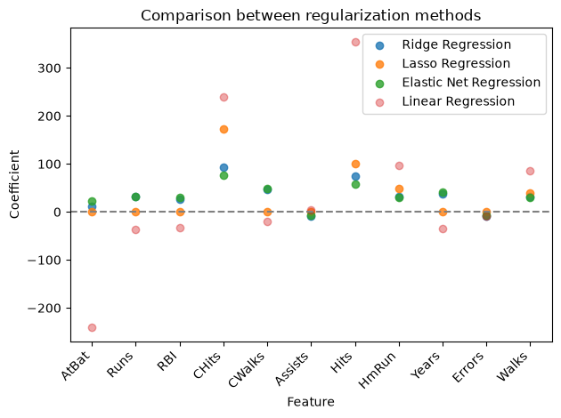
As a summary, we can look at coefficients estimated by all introduced methods:
Now it’s your turn: Head to the exercise section for Exercise 2, in which you will implement a Lasso model.