⚖️ Bias-Variance Tradeoff - Statistical Learning with Python

Before we dive into the concept of bias, let’s briefly recap some theoretical concepts you learned about in the lecture. When we talk about fitting machine learning models, we are referring to the process of estimating a function $f$ that best represents the relationship between an outcome and a set of labelled data (in supervised learning) or to uncover structural patterns in unlabelled data (in unsupervised learning). While the estimated function $\hat{f}$ conveys important information about the data from which it was derived (the training data), our primary interest is in using this function to make accurate predictions for future cases in new, unseen data sets.

The fundamental question in statistical learning is how well $\hat{f}$ will perform on these future data sets, which brings us to the concept of the bias-variance tradeoff. Bias occurs when a model is too simple to capture the underlying complexities of the data, leading to systematic inaccuracies in its predictions. Variance measures how much the model’s predictions fluctuate when trained on different subsets of the data.

This closely relates to the example introduced in 🔁 Recap: Regression Models. Let’s have another look and simulate some data with an underlying relationship in line with a cubic polynomial function. We can see that a linear regression does not capture the nuance of the cubic relationship in the data, while a 10th order model already overfits quite a lot:

import numpy as np

x = np.linspace(-3, 3, 30)
y = (x**3 + np.random.normal(0, 15, size=x.shape)) / 10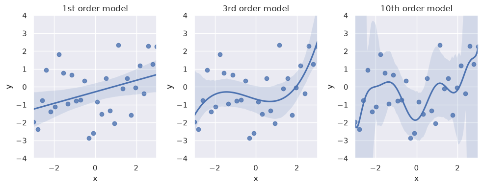

import numpy as np
import pandas as pd
from matplotlib import pyplot as plt
import seaborn as sns

sns.set_theme()
np.random.seed(42)

x = np.linspace(-3, 3, 30)
y = (x**3 + np.random.normal(0, 15, size=x.shape)) / 10
df = pd.DataFrame({'x': x, 'y': y})

fig, ax = plt.subplots(1, 3, figsize=(10, 4))
sns.regplot(df, x="x", y="y", ax=ax[0], order=1)
sns.regplot(df, x="x", y="y", ax=ax[1], order=3)
sns.regplot(df, x="x", y="y", ax=ax[2], order=10)

titles = ["1st order model", "3rd order model", "10th order model"]
for a, title in zip(ax, titles):
    a.set(title=title)
    a.set_xlim(-3, 3)
    a.set_ylim(-4, 4)

plt.tight_layout()

If we look at the mean squared error (MSE) on the training data, we can see that it decreases with increasing model flexibility:

import statsmodels.api as sm
from sklearn.preprocessing import PolynomialFeatures

# Create data
np.random.seed(42)
x = np.linspace(-3, 3, 30).reshape(-1, 1)
y = (x**3 + np.random.normal(0, 15, size=x.shape)) / 10

# Run the models and calculate the MSE
mse_list = []
model_list = []
degrees = [1, 3, 10]

for degree in degrees:
    x_trans = PolynomialFeatures(degree=degree).fit_transform(x)
    model = sm.OLS(y, x_trans).fit()
    mse = np.mean(model.resid**2)

    model_list.append(model)
    mse_list.append(mse)

print("Degree  Train MSE")
for degree, mse in zip(degrees, mse_list):
    print(f"{degree:<7} {mse:.3f}")

Degree  Train MSE
1       1.809
3       1.417
10      1.094

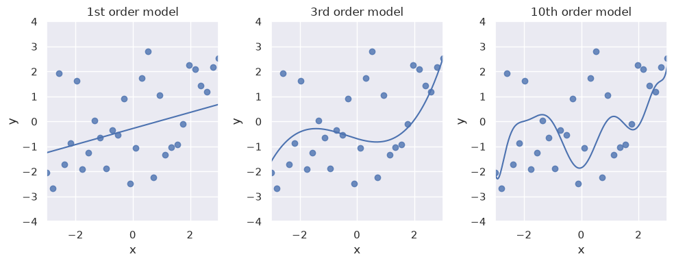
However, if we evaluate the same models on new, unseen data, we see that the MSE is now increasing with increasing order of the polynomial regression model:

# Create data
np.random.seed(42)
x_train = np.linspace(-3, 3, 30)
y_train = (x_train**3 + np.random.normal(0, 15, size=x_train.shape)) / 10

np.random.seed(5)
x_test = np.linspace(-3, 3, 30)
y_test = (x_test**3 + np.random.normal(0, 15, size=x_test.shape)) / 10
df_test = pd.DataFrame({'x': x_test, 'y': y_test})

# Create plot
fig, ax = plt.subplots(1, 3, figsize=(10, 4))
orders = [1, 3, 10]
titles = ["1st order model", "3rd order model", "10th order model"]
predictions = []

for a, order, title in zip(ax, orders, titles):
    coeffs = np.polyfit(x_train, y_train, order)
    x_fit = np.linspace(-5, 5, 400)
    y_fit = np.polyval(coeffs, x_fit)
    y_pred = np.polyval(coeffs, x_test)
    predictions.append(y_pred)

    sns.regplot(data=df_test, x="x", y="y", ax=a, fit_reg=False)
    a.plot(x_fit, y_fit, color='#4c72b0')

    a.set(title=title)
    a.set_xlim(-3, 3)
    a.set_ylim(-4, 4)

plt.tight_layout()
plt.show()

# Calculate the test MSE
mses = [np.mean((pred - y_test)**2) for pred in predictions]

print("Degree  Test MSE")
for order, mse in zip(orders, mses):
    print(f"{order:<7} {mse:.3f}")

Degree  Test MSE
1       2.203
3       2.046
10      2.478

Please compare the previous plots and outputs. What do you notice?

This is because the 10th order model has too much variance — it is too close to the training data. If we fit such a model to multiple draws of samples from the population with a true association consistent with the cubic order polynomial, the model’s predictive performance will always look different:

seeds = [42, 43, 44]
fig, ax = plt.subplots(1, 3, figsize=(10, 4))

for a, seed in zip(ax, seeds):
    np.random.seed(seed)
    x = np.linspace(-3, 3, 30)
    y = (x**3 + np.random.normal(0, 15, size=x.shape)) / 10
    df = pd.DataFrame({'x': x, 'y': y})

    sns.regplot(data=df, x="x", y="y", ax=a, order=10)
    a.set(title=f"Random seed {seed}")
    a.set_xlim(-3, 3)
    a.set_ylim(-4, 4)

plt.tight_layout()
plt.show()

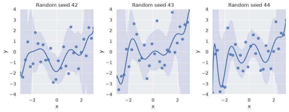
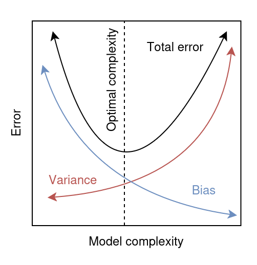
Bias-variance tradeoff — Figure 1:The bias-variance tradeoff.

When we increase the flexibility of the model by adding more parameters, we are effectively trading between bias and variance. Initially, as the model becomes more flexible, its bias decreases quickly because it can capture more complex patterns in the data. However, this increased flexibility also makes the model more sensitive to the noise in the training data, which leads to a rise in variance.

Eventually, the reduction in bias is no longer sufficient to counterbalance the increase in variance. This is why a model with a very low training MSE may still suffer from a high test MSE: the low training error is primarily a result of fitting the noise (i.e. high variance), rather than capturing a true underlying pattern.

Decomposing the error yourself¶

The figure above is usually drawn on a whiteboard and taken on faith. Because we simulated the data, we actually know the true function, so we can measure bias and variance instead of asserting them.

The recipe is simple: draw many training sets from the same population, fit a model of a given degree to each of them, and then look at the predictions at a fixed test point $x_0$ :

Bias² is how far the average prediction is from the truth: $\left(\mathbb{E}[\hat{f}(x_0)] - f(x_0)\right)^2$
Variance is how much the individual predictions scatter around that average: $\mathrm{Var}[\hat{f}(x_0)]$
Irreducible error is the noise variance $\sigma^2$ , which no model can remove

Their sum is the expected test MSE:

\mathbb{E}\left[(y_0 - \hat{f}(x_0))^2\right] = \underbrace{\mathrm{Bias}^2[\hat{f}(x_0)]}_{\text{too simple}} + \underbrace{\mathrm{Var}[\hat{f}(x_0)]}_{\text{too flexible}} + \underbrace{\sigma^2}_{\text{noise}}

(2)

import numpy as np

rng = np.random.default_rng(0)

# The true function and the noise level we simulate from
f_true = lambda x: x**3 / 10
sigma = 1.5
n_train = 30
n_sims = 400
degrees = np.arange(1, 13)

x_grid = np.linspace(-3, 3, 60)          # test points
f_grid = f_true(x_grid)

bias2, variance = [], []

for degree in degrees:
    # Each row holds the predictions of one model, fitted to one simulated dataset
    preds = np.empty((n_sims, x_grid.size))

    for s in range(n_sims):
        x_s = np.linspace(-3, 3, n_train)
        y_s = f_true(x_s) + rng.normal(0, sigma, size=n_train)
        preds[s] = np.polyval(np.polyfit(x_s, y_s, degree), x_grid)

    mean_pred = preds.mean(axis=0)
    bias2.append(np.mean((mean_pred - f_grid) ** 2))
    variance.append(np.mean(preds.var(axis=0)))

bias2 = np.array(bias2)
variance = np.array(variance)
total = bias2 + variance + sigma**2

for d, b, v, t in zip(degrees, bias2, variance, total):
    print(f"degree {d:>2}   bias² = {b:6.3f}   variance = {v:7.3f}   expected test MSE = {t:7.3f}")

degree  1   bias² =  0.184   variance =   0.151   expected test MSE =   2.585
degree  2   bias² =  0.186   variance =   0.192   expected test MSE =   2.628
degree  3   bias² =  0.000   variance =   0.291   expected test MSE =   2.541
degree  4   bias² =  0.002   variance =   0.360   expected test MSE =   2.611
degree  5   bias² =  0.001   variance =   0.408   expected test MSE =   2.659
degree  6   bias² =  0.001   variance =   0.509   expected test MSE =   2.761
degree  7   bias² =  0.001   variance =   0.558   expected test MSE =   2.809
degree  8   bias² =  0.002   variance =   0.632   expected test MSE =   2.884
degree  9   bias² =  0.001   variance =   0.695   expected test MSE =   2.946
degree 10   bias² =  0.004   variance =   0.784   expected test MSE =   3.037
degree 11   bias² =  0.003   variance =   0.884   expected test MSE =   3.136
degree 12   bias² =  0.002   variance =   0.955   expected test MSE =   3.207

fig, ax = plt.subplots(figsize=(7, 4.5))
ax.plot(degrees, bias2, "o-", label="Bias²")
ax.plot(degrees, variance, "o-", label="Variance")
ax.axhline(sigma**2, color="grey", ls=":", label="Irreducible error $\\sigma^2$")
ax.plot(degrees, total, "o-", color="k", lw=2, label="Expected test MSE")

best = degrees[np.argmin(total)]
ax.axvline(best, color="crimson", ls="--", alpha=0.6)
ax.annotate(f"best degree = {best}", xy=(best, total.max() * 0.8),
            xytext=(best + 0.4, total.max() * 0.85), color="crimson")

ax.set(xlabel="Polynomial degree (model flexibility)", ylabel="Error",
       title="Measured bias-variance decomposition", xticks=degrees)
ax.set_yscale("log")
ax.legend()
plt.tight_layout()

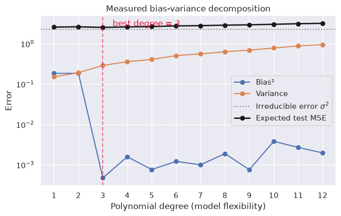
Notice that the measured curve has exactly the shape of the schematic figure: bias² collapses as soon as the model is flexible enough to represent a cubic, variance grows steadily, and their sum has a minimum at degree 3 — the degree we actually simulated from. The expected test MSE never drops below $\sigma^2 = 2.25$ , no matter how good the model gets.