One of the most important concepts in any multivariate statistics seminar such as psy111 are (linear) regression models. Let’s quickly recap this concept and how to implement it in Python.
Have a look at the following code, which creates some simulated data. Can you deduce from the code what the underlying pattern is?
import numpy as np
import pandas as pd

x = np.linspace(-5, 5, 30)
y = (x**3 + np.random.normal(0, 15, size=x.shape)) / 50

df = pd.DataFrame({'x': x, 'y': y})
Click to reveal the plot
Here you can see the data in a scatterplot, with a linear regression model fitted to the data. Do you think the linear model fits the data well?
Let’s take a closer look at the model. As introduced last semester, we can e.g. use the statsmodels.formula.api library to specify and fit regression models with a formula notation similar to R. We use the ols() class to fit the model specified as y ~ x, which translates to “y predicted by x”:
import statsmodels.formula.api as smf

model = smf.ols("y ~ x", data=df).fit()
print(model.summary())
OLS Regression Results
==============================================================================
Dep. Variable: y R-squared: 0.753
Model: OLS Adj. R-squared: 0.745
Method: Least Squares F-statistic: 85.59
Date: Wed, 12 Aug 2026 Prob (F-statistic): 5.21e-10
Time: 14:15:57 Log-Likelihood: -21.439
No. Observations: 30 AIC: 46.88
Df Residuals: 28 BIC: 49.68
Df Model: 1
Covariance Type: nonrobust
==============================================================================
coef std err t P>|t| [0.025 0.975]
------------------------------------------------------------------------------
Intercept -0.0564 0.093 -0.604 0.551 -0.248 0.135
x 0.2896 0.031 9.251 0.000 0.226 0.354
==============================================================================
Omnibus: 1.772 Durbin-Watson: 0.635
Prob(Omnibus): 0.412 Jarque-Bera (JB): 1.169
Skew: 0.183 Prob(JB): 0.557
Kurtosis: 2.105 Cond. No. 2.98
==============================================================================
Notes:
[1] Standard Errors assume that the covariance matrix of the errors is correctly specified.
In this output, the most important information are the model parameters displayed under coef and the performance statistics such as the R-squared.
You can see that our model has an R-squared of 0.753, which means that the model explains 75% of the variance in the data. That’s pretty good! But I’m sure we can do better. After all, life is more complicated than just a straight line, no? (And we also know that the underlying data was simulated according to a 3rd order polynomial.)
Drag the slider below to increase the order of the polynomial and watch the R² climb:
As you probably expected, the R² increases as you increase the order of the polynomial in the regression model. However, this doesn’t stop after the 3rd order polynomial (which is the true function that generated the data). The R² continues to increase until it hits 1 for a model that includes a 29th-order polynomial. You can see that the model now goes through every single one of the data points. This did not happen by chance! A polynomial of degree 29 can perfectly interpolate the present data, which consists of 30 data points. This is because a polynomial of degree has coefficients, which can be uniquely determined to pass through distinct points (given that all the x-values are distinct).
But what should you do with this information? Well, as the topic of this seminar is statistical and machine learning, we are usually concerned with making predictions for new, unseen data. Until now, we have always fit (trained) and evaluated (tested) our model on the same data, aiming to make statistical inferences about the coefficients of relatively small models. We can call this the training data[1]. However, we can also generate new data with the same underlying function and test the model on this repeatedly generated data that reflects the same underlying true association between y and x. We call this the testing data[2]:
You can see that the R² now has a peak around a 3rd order polynomial regression model and then drastically decreases for higher order polynomials. This means that our previously trained models do not really fit our new data anymore. Why is this the case? Basically, these higher-order models became too flexible and overfit[3] to the training data. Once we apply the models to new testing data, they will produce a much worse performance, as they are too specialized (they basically just memorized the training data).
So how can we then find the best model that avoids overfitting? From your classes in basic (psychological) methods, you might be familiar with Occam’s razor, which states that:
Entia non sunt multiplicanda praeter necessitatem.
This essentially translates to “Before you try a complicated hypothesis, you should make quite sure that no simplification of it will explain the facts equally well”. Our model should thus be as simple as possible, but as complex as necessary. In machine learning, this concept is often referred to as the bias-variance tradeoff, which we will explore next week.
Different Ways of Implementing Regression Models
There are many different Python packages that allow you to implement regression models, with popular choices being statsmodels, numpy, and sklearn. The specific choice ultimately depends on your preferences and goals.
At the top of this section, you have already seen the high-level formula API solution from statsmodels. For a cubic model, this would look like this:
import statsmodels.formula.api as smf

# Fit model
model = smf.ols("y ~ x + I(x**2) + I(x**3)", data=df).fit()

# Predictions
x_new = pd.DataFrame({"x": [-4, 1, 3]})
print(model.predict(x_new))
0 -1.149150
1 -0.148156
2 0.380523
dtype: float64
Alternatively, you can use the lower-level OLS() approach, which requires you to manually specify the design matrix (make sure to add a column for the intercept/bias):
import statsmodels.api as sm
from sklearn.preprocessing import PolynomialFeatures

# Create design matrix
X = x.reshape(-1, 1)
poly = PolynomialFeatures(degree=3, include_bias=True)
X_poly = poly.fit_transform(X)

# Fit model
model = sm.OLS(y, X_poly).fit()
A cool thing about statsmodels is that you can get the model results in various forms:
summary = model.summary()
print(summary)
OLS Regression Results
==============================================================================
Dep. Variable: y R-squared: 0.943
Model: OLS Adj. R-squared: 0.936
Method: Least Squares F-statistic: 143.0
Date: Wed, 12 Aug 2026 Prob (F-statistic): 2.83e-16
Time: 14:15:58 Log-Likelihood: 0.48444
No. Observations: 30 AIC: 7.031
Df Residuals: 26 BIC: 12.64
Df Model: 3
Covariance Type: nonrobust
==============================================================================
                 coef    std err          t      P>|t|      [0.025      0.975]
------------------------------------------------------------------------------
const         -0.1381      0.070     -1.969      0.060      -0.282       0.006
x1            -0.0398      0.039     -1.014      0.320      -0.121       0.041
x2             0.0092      0.006      1.561      0.131      -0.003       0.021
x3             0.0206      0.002      9.148      0.000       0.016       0.025
==============================================================================
Omnibus: 1.544 Durbin-Watson: 2.234
Prob(Omnibus): 0.462 Jarque-Bera (JB): 1.008
Skew: 0.449 Prob(JB): 0.604
Kurtosis: 2.975 Cond. No. 78.5
==============================================================================
Notes:
[1] Standard Errors assume that the covariance matrix of the errors is correctly specified.
print(summary.tables[1])==============================================================================
coef std err t P>|t| [0.025 0.975]
------------------------------------------------------------------------------
const -0.1381 0.070 -1.969 0.060 -0.282 0.006
x1 -0.0398 0.039 -1.014 0.320 -0.121 0.041
x2 0.0092 0.006 1.561 0.131 -0.003 0.021
x3 0.0206 0.002 9.148 0.000 0.016 0.025
==============================================================================
print(model.params) # [beta0, beta1, beta2, beta3][-0.13806828 -0.03982915 0.00916298 0.02057822]
# Prediction
x_new = np.array([[-4], [1], [3]])
X_new_poly = poly.transform(x_new)
y_hat = model.predict(X_new_poly)
print(y_hat)
[-1.14914986 -0.14815624 0.38052287]
With the polynomial features, we can also directly use sklearn:
from sklearn.linear_model import LinearRegression

# Fit model
model = LinearRegression(fit_intercept=False).fit(X_poly, y)  # the intercept is already in X_poly
print(model.coef_)  # [beta0, beta1, beta2, beta3]

# Predict
y_hat = model.predict(X_new_poly)
print(y_hat)
[-0.13806828 -0.03982915 0.00916298 0.02057822]
[-1.14914986 -0.14815624 0.38052287]
And last but not least, one could also use numpy:
import numpy as np
from matplotlib import pyplot as plt

coeffs = np.polyfit(x, y, deg=3)
print(coeffs)
p = np.poly1d(coeffs)

# Predict
x_new = np.array([-4, 1, 3])
y_hat = p(x_new)
print(y_hat)

# Plot
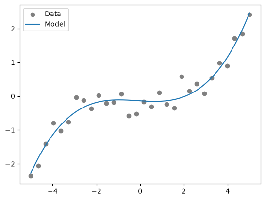
fig, ax = plt.subplots()
ax.scatter(x, y, color="gray", label="Data")
x_fit = np.linspace(x.min(), x.max(), 200)
ax.plot(x_fit, p(x_fit), label="Model")
plt.legend();
[ 0.02057822 0.00916298 -0.03982915 -0.13806828]
[-1.14914986 -0.14815624 0.38052287]
In practice, statsmodels is ideal for statistical analysis and reporting (it provides a lot of information for inference), scikit-learn for machine learning pipelines and prediction, and numpy for quick or lightweight fits.
Training data refers to the data which was used for model fitting.
Testing data refers to data which was used to evaluate the performance of a model. This is new, unseen data, meaning that it was not used for training.
Overfitting refers to fitting patterns in the training data which do not generalize to the testing data.