As future data scientists, you are probably well aware of the challenges involved in data collection — time, cost, and the complexities of experimental design often make large datasets hard to come by. However, robust predictive modeling is critical not only because extensive datasets can be rare, but also because ensuring that models generalize well to new data is often an essential question.
Resampling methods offer a powerful approach to assess model performance and mitigate overfitting. Rather than relying on a single train-test split, which can yield performance estimates that vary significantly depending on the split, resampling techniques repeatedly draw samples from your data. This process simulates multiple independent training and test sets, providing a more stable and reliable evaluation of your model.
The data
We will use the famous Iris dataset, which contains 150 samples from three species of the iris plant (iris setosa, iris virginica and iris versicolor). The data contains four features: the length and the width of the sepals and petals (in centimeters).
import seaborn as sns
import pandas as pd
from sklearn import datasets

# Get data
iris = datasets.load_iris(as_frame=True)
df = iris.frame
df['class'] = pd.Categorical.from_codes(iris.target, iris.target_names)

df.describe()sns.scatterplot(data=df, x='sepal length (cm)', y='sepal width (cm)', hue="class");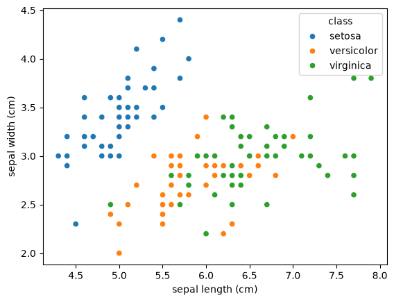
The goal of our model is to classify the flowering plants based on the two features shown in the plot (sepal length and width). Which of the following is true about the model and task at hand?
Validation Sets
The simplest form of cross-validation is to simply split the dataset into two parts:
Training set: part of the data used for training
Validation set: part of the data used for testing (e.g. across different models and hyperparameters)
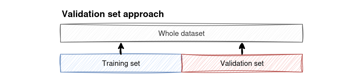
Figure 1:The validation set splits the dataset into a training and a testing set (these do not necessarily need to be of equal size).
The training and testing set neither need to be of equal size nor do they need to be contiguous blocks in the data. Let’s try the validation set approach on the Iris data:
Define features and target data
# Features: sepal length and width; target: type of flower
X = df[["sepal length (cm)", "sepal width (cm)"]]
y = df["target"]
Split the data into training and test samples
from sklearn.model_selection import train_test_split

X_train, X_test, y_train, y_test = train_test_split(X, y, test_size=0.4, random_state=42)
Fit the model (we use a support vector classifier which you will learn about later in the seminar)
from sklearn import svm

model = svm.SVC(kernel='linear')
fit = model.fit(X_train, y_train)
Evaluate model performance
fit.score(X_test, y_test)0.85The score() method returns the accuracy of our predictions. In this case, our algorithm correctly predicted the species of the flower in 85% of cases.
How much does that 85% actually mean?
The number above came out of exactly one split, chosen by random_state=42. Nothing about 42 is special. So what happens if we repeat the same procedure with 500 different random splits?
Source
import numpy as np
import matplotlib.pyplot as plt

split_scores = []
for seed in range(500):
    X_tr, X_te, y_tr, y_te = train_test_split(X, y, test_size=0.4, random_state=seed)
    split_scores.append(svm.SVC(kernel='linear').fit(X_tr, y_tr).score(X_te, y_te))

split_scores = np.array(split_scores)

fig, ax = plt.subplots(figsize=(7, 4))
ax.hist(split_scores, bins=25, color="#4c72b0", alpha=0.8)
ax.axvline(split_scores.mean(), color="k", ls="--",
           label=f"mean = {split_scores.mean():.3f}")
ax.axvline(split_scores[42], color="crimson", lw=2,
           label=f"random_state=42 → {split_scores[42]:.3f}")
ax.set(xlabel="Test accuracy", ylabel="Number of splits",
       title="Accuracy of 500 different validation-set splits")
ax.legend()
plt.tight_layout()

print(f"mean  {split_scores.mean():.3f}")
print(f"std   {split_scores.std():.3f}")
print(f"range {split_scores.min():.3f} – {split_scores.max():.3f}")
mean 0.792
std 0.044
range 0.633 – 0.917
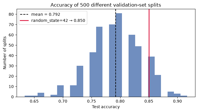
The spread is remarkable. Depending on nothing but the random seed, the very same model looks anywhere from clearly mediocre to surprisingly good. Reporting a single split as the performance of your model is therefore reporting a coin flip.
Try it yourself: the split ratio matters too. Before running the cell below, think about what you expect: is it better to train on 80% of the data and test on 20%, or the other way round? Then change test_size and see whether the result matches your intuition.
for test_size in [0.2, 0.5, 0.8]:
    X_tr, X_te, y_tr, y_te = train_test_split(X, y, test_size=test_size, random_state=42)
    acc = svm.SVC(kernel='linear').fit(X_tr, y_tr).score(X_te, y_te)
    print(f"train on {1 - test_size:.0%} / test on {test_size:.0%}"
          f"   ->   {len(X_tr):>3} training samples, accuracy = {acc:.3f}")
train on 80% / test on 20% -> 120 training samples, accuracy = 0.900
train on 50% / test on 50% -> 75 training samples, accuracy = 0.760
train on 20% / test on 80% -> 30 training samples, accuracy = 0.775
Training on more data generally gives a better model, but it also leaves fewer test samples, so the accuracy estimate itself becomes noisier. That is the tradeoff the validation set approach cannot escape.
Cross-Validation (CV)
K-fold CV
To get more robust performance estimates, we need something smarter. Rather than worrying about whether the split of data used for training and validation is biased, we will perform this splitting multiple times and use all of the splits in turn.
In k-fold CV we randomly divide the dataset into equally sized folds. In each round, one fold is designated as the validation set, while the remaining folds form the training set. The fitting process is repeated times, each time using a different fold as the validation set. At the end of the process, we can compute the average accuracy across all validation folds to obtain a more reliable estimate of the model’s overall performance.
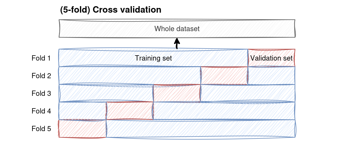
Figure 2:K-fold cross-validation splits the dataset into equally sized parts and then trains the model on all possible combinations of them, keeping the proportion of train/test data constant.
Let’s try it on our data:
from sklearn.model_selection import KFold, cross_val_score

k_fold = KFold(n_splits=5, shuffle=True, random_state=42)
model = svm.SVC(kernel='linear')

scores = cross_val_score(model, X, y, cv=k_fold)

print(f"Average accuracy:      {scores.mean():.3f}")
print(f"Individual accuracies: {np.round(scores, 3)}")
Average accuracy: 0.807
Individual accuracies: [0.9 0.767 0.767 0.833 0.767]
Try it and watch what happens:
scores_unshuffled = cross_val_score(model, X, y, cv=KFold(n_splits=5))
print(f"Without shuffling: {np.round(scores_unshuffled, 3)} → mean {scores_unshuffled.mean():.3f}")
Without shuffling: [1. 0.8 0.3 0.767 0.2 ] → mean 0.613
That 0.61 is not a property of the model — it is an artefact of the row ordering. Whenever your data has any kind of structure in its row order (sorted by group, collected by session, ordered in time), shuffling or a grouped/stratified splitter matters more than the choice of .
For classification it is usually even better to use StratifiedKFold, which additionally keeps the class proportions constant in every fold. In fact, if you pass a plain integer to cross_val_score, scikit-learn does this for you automatically:
# cv=5 with a classifier → StratifiedKFold under the hood
scores_stratified = cross_val_score(svm.SVC(kernel='linear'), X, y, cv=5)
print(f"Average accuracy: {scores_stratified.mean():.3f}")
Average accuracy: 0.807
If we are interested in the individual models, we can also run the training and evaluation explicitly, which allows us to save them:
from sklearn.base import clone

base_model = svm.SVC(kernel='linear')
score_list = []
model_list = []

for train_index, test_index in k_fold.split(X):
    X_train, X_test = X.iloc[train_index], X.iloc[test_index]  # iloc because X is a DataFrame
    y_train, y_test = y.iloc[train_index], y.iloc[test_index]  # iloc because y is a Series

    model = clone(base_model)  # create a new copy of the model for every iteration
    model.fit(X_train, y_train)
    score = model.score(X_test, y_test)

    score_list.append(score)
    model_list.append(model)

print(f"Best performing model in split {score_list.index(max(score_list))}.")
print(f"Accuracy: {max(score_list):.3f}")
Best performing model in split 0.
Accuracy: 0.900
Try it yourself: change the number of folds below and watch what happens. What do you feel is a good tradeoff?
for k in [2, 5, 10, 20, 50]:
    cv = KFold(n_splits=k, shuffle=True, random_state=42)
    s = cross_val_score(svm.SVC(kernel='linear'), X, y, cv=cv)
    print(f"k = {k:>2}   mean accuracy = {s.mean():.3f}   "
          f"std across folds = {s.std():.3f}   ({k} model fits)")
k = 2 mean accuracy = 0.760 std across folds = 0.000 (2 model fits)
k = 5 mean accuracy = 0.807 std across folds = 0.053 (5 model fits)
k = 10 mean accuracy = 0.787 std across folds = 0.111 (10 model fits)
k = 20 mean accuracy = 0.806 std across folds = 0.122 (20 model fits)
k = 50 mean accuracy = 0.813 std across folds = 0.242 (50 model fits)
Notice that the mean barely moves once , while the standard deviation across folds keeps growing — with more folds each test set is smaller, so each individual fold score is noisier even though their average is stable. The extra compute buys you very little beyond or 10.
Leave-one-out CV (LOOCV)
LOOCV is a special case of k-fold cross-validation, where equals the number of observations. In LOOCV, the model is trained on all but one data point, and the remaining single observation is used for validation. This process repeats for each data point, ensuring every observation is used for testing exactly once.
While LOOCV provides a low-bias estimate, it is computationally expensive and the individual fold scores are extremely coarse — with a single test point, each fold score can only ever be 0 or 1. The implementation is fairly similar, we just need to change the CV splitter from KFold() to LeaveOneOut():
from sklearn.model_selection import LeaveOneOut

model = svm.SVC(kernel='linear')
loocv = LeaveOneOut()

scores = cross_val_score(model, X, y, cv=loocv)

print(f"Average accuracy:      {scores.mean():.3f}")
print(f"Individual accuracies: {np.unique(scores)}  (only 0 or 1 possible)")
print(f"Number of fits:        {len(scores)}")
Average accuracy: 0.800
Individual accuracies: [0. 1.] (only 0 or 1 possible)
Number of fits: 150
Bootstrapping
Bootstrapping is a resampling method that helps us estimate how much a model’s results might vary if we collected a different dataset. The idea is simple: instead of having just one training set, we create many “new” datasets by sampling with replacement from the original data.
Each bootstrap sample is the same size as the original dataset, but because sampling is done with replacement, some observations will appear more than once, while others might not appear at all.
For each bootstrap iteration:
A new sample (the bootstrap sample) is drawn from the data.
The model is trained on this bootstrap sample.
The observations that were not included in that sample — called out-of-bag (OOB) samples — are used to test the model.
Repeating this process many times gives multiple estimates of model performance. The variability among these estimates provides insight into the model’s uncertainty and stability. In contrast, cross-validation divides the data into fixed folds and does not resample with replacement. Cross-validation is generally better for estimating predictive accuracy, while bootstrapping is often used to assess the uncertainty of model parameters or performance estimates.
We here outline the concept with 10 iterations:
import numpy as np
import pandas as pd
from sklearn import datasets, svm
from sklearn.utils import resample

# Load the data
iris = datasets.load_iris(as_frame=True)
df = iris.frame

n_iterations = 10
scores = []

for i in range(n_iterations):
    # Create a bootstrap sample
    bootstrap_sample = resample(df, replace=True, n_samples=len(df), random_state=i)

    # Determine the out-of-bag (OOB) samples: rows not in the bootstrap sample
    oob_indices = df.index.difference(bootstrap_sample.index)

    # If no OOB samples are available, skip this iteration
    if len(oob_indices) == 0:
        print(f"Iteration {i+1}: No out-of-bag samples, skipping iteration.")
        continue

    oob_sample = df.loc[oob_indices]

    # Define features and target for training and testing
    X_train = bootstrap_sample[["sepal length (cm)", "sepal width (cm)"]]
    y_train = bootstrap_sample["target"]
    X_test = oob_sample[["sepal length (cm)", "sepal width (cm)"]]
    y_test = oob_sample["target"]

    # Train and evaluate the model
    model = svm.SVC(kernel='linear')
    model.fit(X_train, y_train)

    score = model.score(X_test, y_test)
    scores.append(score)
    print(f"Iteration {i+1}: Accuracy = {score:.3f}")

print(f"\nMean OOB accuracy: {np.mean(scores):.3f}")
Iteration 1: Accuracy = 0.774
Iteration 2: Accuracy = 0.825
Iteration 3: Accuracy = 0.759
Iteration 4: Accuracy = 0.817
Iteration 5: Accuracy = 0.818
Iteration 6: Accuracy = 0.778
Iteration 7: Accuracy = 0.827
Iteration 8: Accuracy = 0.729
Iteration 9: Accuracy = 0.807
Iteration 10: Accuracy = 0.839
Mean OOB accuracy: 0.797
The OOB estimate lands very close to the shuffled 5-fold estimate. That is the expected outcome: both are honest estimates of the same generalisation performance, computed on data the model never saw during training.
Source
# How many distinct observations does a bootstrap sample actually contain?
n = len(df)
unique_fractions = [
    len(np.unique(resample(np.arange(n), replace=True, n_samples=n, random_state=i))) / n
    for i in range(200)
]
print(f"Mean fraction of distinct observations: {np.mean(unique_fractions):.3f}")
print(f"Theoretical value 1 - (1 - 1/n)^n:      {1 - (1 - 1/n)**n:.3f}")
Mean fraction of distinct observations: 0.636
Theoretical value 1 - (1 - 1/n)^n: 0.633