Please fill the missing code pieces as indicated by the .... The imports are always provided at the top of the code chunks. This should give you a hint for which functions/classes to use. Have a look at the online documentation if you are unsure how to use them.
Exercise 1: Model Selection
We are working with the California Housing dataset again, which you already know from the resampling session. It is based on the 1990 U.S. Census and contains features describing districts in California.
Load the data and extract the features (
X) and the target (y)
from sklearn.datasets import fetch_california_housing

# TODO: Get data
...

# TODO: Extract features and target
...
Baseline model
Split the data into 80% training and 20% test data (print the shapes to confirm that it was successful)
Evaluate a linear regression with all features on the training data, using 5-fold cross-validation and R² as the performance metric. Remember what you learned about shuffling in the resampling session!
Print the individual and the average R²
import numpy as np
from sklearn.linear_model import LinearRegression
from sklearn.model_selection import train_test_split, KFold, cross_val_score

# TODO: Split data into training and test sets
...

# TODO: Evaluate the baseline model with 5-fold cross-validation
...
Apply forward stepwise selection to find a simpler model
Use a linear regression model, the same cross-validation folds as for the baseline, R² as the score, and
k_features="parsimonious". This option picks the smallest subset whose CV score is within one standard error of the best subset (see the documentation)Print the best CV R² as well as the chosen features. How does the CV R² compare to the baseline?
from mlxtend.feature_selection import SequentialFeatureSelector

# TODO: Perform forward sequential feature selection
sfs_forward = ...

# Summary of results
print(f">> Forward SFS:")
print(f"   Best CV R²      : {sfs_forward.k_score_:.3f}")
print(f"   Optimal # feats : {len(sfs_forward.k_feature_idx_)}")
print(f"   Feature names   : {sfs_forward.k_feature_names_}")
Evaluate both the baseline model and the selected model on the test set. Is the simpler model worse?
# TODO: Get the selected features as a list
...

# TODO: Train both models on the training data and evaluate them on the test set
...
Exercise 2: Lasso
Please implement a Lasso regression model similar to the Ridge model in the Regularization section:
Prepare the data: drop the highly correlated features and rows with missing data, split the data into training and test set, and scale the predictors
Use
LassoCVwith 5-fold cross-validation to find the optimal λ. Test 100 values between 0.01 and 1000, evenly spaced on a log scale (np.logspace())Print the optimal λ, the training and test R², and the coefficients. Which predictors does Lasso remove?
Is the optimal λ at the edge of the range you tested? Why would that be a problem?
import pandas as pd
import numpy as np
import statsmodels.api as sm

from sklearn.preprocessing import StandardScaler
from sklearn.linear_model import LassoCV
from sklearn.model_selection import train_test_split

# Data related processing
hitters = sm.datasets.get_rdataset("Hitters", "ISLR").data
hitters_subset = hitters[["Salary", "AtBat", "Runs","RBI", "CHits", "CAtBat", "CRuns", "CWalks", "Assists", "Hits", "HmRun", "Years", "Errors", "Walks"]].copy()

# TODO: Drop highly correlated features and rows with missing data
...

# TODO: Get the target (y) and features (X), then split into training and test set
...

# TODO: Scale predictors to mean=0 and std=1
...

# TODO: Find the optimal lambda with LassoCV
...

# TODO: Print the optimal lambda, the training and test R², and the coefficients
...
Exercise 3: Principal Component Analysis
In this exercise, we work with the Diabetes dataset from scikit-learn. It contains 10 baseline measurements of 442 diabetes patients: age, sex, body mass index (bmi), average blood pressure (bp), and six blood serum measurements (s1 to s6). The target is a measure of disease progression one year after baseline. You can read more in the documentation or with print(diabetes.DESCR).
Inspect the data
Use
.describe()and.isna().sum()to get summary statistics and to check for missing valuesLook at the mean and the standard deviation of the features. What do you notice? (Hint:
print(diabetes.DESCR))
from sklearn.datasets import load_diabetes

# Load the data as a DataFrame
diabetes = load_diabetes(as_frame=True)
X = diabetes.data
y = diabetes.target

# TODO: Inspect the data and check for missing values
...
Fit a PCA
Standardize the features with
StandardScaler()and fit aPCA()with all componentsPlot the explained variance ratio of each component (scree plot, e.g. as bars) and the cumulative explained variance (line) next to each other
How many components do you need to explain at least 80% of the variance? Is there a clear elbow?
import numpy as np
import matplotlib.pyplot as plt
from sklearn.preprocessing import StandardScaler
from sklearn.decomposition import PCA

# TODO: Standardize the data and fit the PCA
X_std = ...
pca = ...

# TODO: Plot the explained variance ratio and the cumulative explained variance
fig, ax = plt.subplots(1, 2, figsize=(12, 4))
...
Interpret the loadings
Create a DataFrame with the loadings of the first three components (one row per component, one column per feature)
Plot it with
sns.heatmap()(useful arguments:annot=True,cmap="coolwarm",center=0)Which features have the largest absolute loadings on PC1 and PC2? What could these components represent? The serum measurements are:
s1total cholesterol,s2LDL (“bad” cholesterol),s3HDL (“good” cholesterol),s4ratio of total cholesterol to HDL,s5triglycerides (log),s6blood sugar
import pandas as pd
import seaborn as sns

# TODO: Create a DataFrame with the loadings of the first three components
loadings = ...

# TODO: Plot the loadings as a heatmap
...
Project the data
Transform the standardized data into the PCA space
Create a scatter plot of PC1 against PC2 and color the points by disease progression (
y)Along which component does the disease progression change? Remember that the PCA never saw
y!
# TODO: Project the data into the PCA space
X_pca = ...

# TODO: Plot PC1 against PC2, colored by disease progression
...
Exercise 3.2: PCR and PLS
Now we use the components to predict disease progression. We continue with the same data (X and y) as in the previous exercise.
Visualize the correlations between the predictors with a heatmap. Which predictors are strongly correlated? Why could this be a problem for a linear regression?
# TODO: Plot the correlation matrix with sns.heatmap()
...
PCR with a range of components
Split the data into 80% training and 20% test data (
random_state=42)Set up a 10-fold cross-validation with shuffling (
random_state=42)For 1 to 10 components, create a PCR pipeline with
make_pipeline()(StandardScaler,PCA,LinearRegression) and evaluate it on the training data withcross_val_score(). Store the mean R² of each model
from sklearn.pipeline import make_pipeline
from sklearn.linear_model import LinearRegression
from sklearn.model_selection import train_test_split, cross_val_score, KFold

# TODO: Split the data and set up the cross-validation
X_train, X_test, y_train, y_test = ...
cv = ...

# TODO: Loop over the number of components, create the pipeline, evaluate it with cross_val_score()
n_components = np.arange(1, X.shape[1] + 1)
pcr_scores = []

for n in n_components:
    model = ...
    scores = ...
    pcr_scores.append(scores.mean())
PLS and comparison
Do the same with
PLSRegression(it standardizes the predictors by itself)As a baseline, also compute the cross-validated R² of a plain linear regression with all predictors
Plot the R² of PCR and PLS over the number of components, and add the baseline as a horizontal line (
ax.axhline())How does PLS compare to PCR?
from sklearn.cross_decomposition import PLSRegression

# TODO: Loop over the number of components, create the PLS model, evaluate it with cross_val_score()
pls_scores = []

for n in n_components:
    pls = ...
    scores = ...
    pls_scores.append(scores.mean())

# TODO: Compute the baseline
lr_score = ...

# TODO: Plot PCR, PLS, and the baseline together
fig, ax = plt.subplots()
...
Why does the PCR performance jump at 4 components?
Fit the first two steps of a PCR pipeline (scaler and PCA with all components) on the training data and compute the scores of the training data
Compute the correlation of each component with
y_train(np.corrcoef()) and compare it to the explained variance ratio of the componentWhat do you notice? How does this relate to the example in the session?
# TODO: Fit the scaler and the PCA on the training data and compute the scores
pca_pipe = ...
scores_train = ...

# TODO: Compute the correlation of each component with y_train
...
Test set evaluation
For PCR and PLS, choose the smallest number of components after which the CV R² hardly improves
Fit both models and the linear regression baseline on the full training data and print their test R²
Was the dimension reduction worth it in this dataset?
# TODO: Fit the final models on the training data and evaluate them on the test set
...
Exercise 4: Logistic Regression
For today’s exercise we will use the Breast Cancer Wisconsin (Diagnostic). It is a collection of data used for predicting whether a breast tumor is malignant (cancerous) or benign (non-cancerous), containing information derived from images of breast mass samples obtained through fine needle aspirates.
The dataset consists of 569 samples with 30 features that measure various characteristics of cell nuclei, such as radius, texture, perimeter, and area. Each sample is labeled as either malignant (1) or benign (0).
Please visit the documentation and familiarize yourself with the dataset
Take an initial look at the features (predictors) and targets (outcomes)
import numpy as np
import matplotlib.pyplot as plt
from ucimlrepo import fetch_ucirepo

# Fetch dataset
breast_cancer_wisconsin_diagnostic = fetch_ucirepo(id=17)

# Get data (as pandas dataframes)
X = ...
y = ...

# Convert y to a 1D array (this is the required input for the logistic regression model)
y = ...

# Print some general information and statistics about the dataset
...
Split the data into training and test sets (stratify
y)Create and fit a baseline model using only 2-3 interpretable predictors of your choice
Print the model coefficients
Evaluate on the test set:
Accuracy
Confusion matrix
Classification report
Compare test accuracy to train accuracy. Is there a big gap?
Hint: If you get a warning about convergence, try setting max_iter=10000 in the logistic regression class.
from sklearn.model_selection import train_test_split
from sklearn.linear_model import LogisticRegression
from sklearn.metrics import accuracy_score, confusion_matrix, classification_report

# 1. Split the data
...

# 2. Baseline model with three features
...

# 3. Evaluate the baseline model
...
Use all predictors and build a pipeline with standardisation
Evaluate on the test set
Compare:
Baseline model vs full model (test accuracy, precision, recall for malignant)
Is the full model clearly better?
Is there any sign of overfitting (train vs test)?
from sklearn.pipeline import Pipeline
from sklearn.preprocessing import StandardScaler

# 4. Full model with all features
...

# 5. Evaluate the full model
...
Create a custom plot which visualizes the confusion matrix It should contain:
The four squares of the matrix (color coded)
Labels of the actual values in the middle of each square
Labels for all squares
A colorbar
A title
Use scikit-learn to do the same
# 6. Plot a custom confusion matrix
...

# 6. Use scikit-learn
from sklearn.metrics import ConfusionMatrixDisplay

...
Exercise 5: LDA, QDA & Naïve Bayes
Once again, we will use the Iris dataset for classificationa analysis. Your task is to compare the performance of LDA, QDA, and Gaussian Naïve Bayes!
Load the
irisdataset fromsklearn.datasets. We will use only the first two features (sepal length and width)TODO:Split the data into training and test sets (use stratification!)TODO:Fit LDA, QDA, and Naïve Bayes classifiers to the training data and orint the classification report for all models on the test dataPlot the decision boundaries for both models
import numpy as np
import matplotlib.pyplot as plt
from sklearn.datasets import load_iris
from sklearn.metrics import classification_report
from sklearn.model_selection import train_test_split
from matplotlib.colors import ListedColormap

# 1. Load data
iris = load_iris()
X = iris.data[:, :2]
y = iris.target
target_names = iris.target_names

# 2. Split into train/test
...
from sklearn.discriminant_analysis import LinearDiscriminantAnalysis
# 3. TODO: Fit a LDA model and print the classification report
lda = ...from sklearn.discriminant_analysis import QuadraticDiscriminantAnalysis
# 3. TODO: Fit a QDA model and print the classification report
qda = ...from sklearn.naive_bayes import GaussianNB
# 3. TODO: Fit a Gaussian Naive Bayes model and print the classification report
gnb = ...Once you have trained all three models, you can plot their decision boundaries based on the training data. For this, you can use the provided helper function below:
# 4. Plot the decision boundaries for all 3 classifiers

# Helper function to plot decision boundaries
def plot_decision_boundary(model, X, y, title, ax):
    h = .02
    x_min, x_max = X[:, 0].min() - .5, X[:, 0].max() + .5
    y_min, y_max = X[:, 1].min() - .5, X[:, 1].max() + .5
    xx, yy = np.meshgrid(np.arange(x_min, x_max, h),
                         np.arange(y_min, y_max, h))
    Z = model.predict(np.c_[xx.ravel(), yy.ravel()])
    Z = Z.reshape(xx.shape)

    cmap_light = ListedColormap(['#FFAAAA', '#AAFFAA', '#AAAAFF'])
    cmap_bold = ListedColormap(['#FF0000', '#00FF00', '#0000FF'])

    ax.contourf(xx, yy, Z, cmap=cmap_light, alpha=0.2)
    scatter = ax.scatter(X[:, 0], X[:, 1], c=y, cmap=cmap_bold, s=30)
    ax.set_xlim(xx.min(), xx.max())
    ax.set_ylim(yy.min(), yy.max())
    ax.set_title(title)
    ax.set_xlabel('Sepal length')
    ax.set_ylabel('Sepal width')

# Create plots for all 3 classifiers
fig, axes = plt.subplots(1, 3, figsize=(12, 4))
...  # LDA
...  # QDA
...  # Naïve Bayes
plt.tight_layout()
Exercise 6: Polynomial and Flexible Regression
In this exercise, we analyse the relationship between wage and age using four flexible regression approaches:
Polynomial regression
Stepwise functions (degree-0 splines)
Spline regression
Local regression (LOWESS)
We will use the Wage dataset for the following exercises. Please briefly visit the documentation for further information: https://
import numpy as np
import matplotlib.pyplot as plt
import statsmodels.api as sm

wage = sm.datasets.get_rdataset("Wage", "ISLR").data

fig, ax = plt.subplots()
ax.scatter(wage["age"], wage["wage"], alpha=0.15)
ax.set(xlabel="Age", ylabel="Wage", title="Wage vs Age");

wage.head()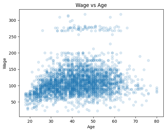
Please predict Wage from Age using four different models:
A polynomial regression model of degree 3
A stepwise model with cut points at 30, 50, and 65 years
A third order spline regression model with
df=6A lowes local regression model with
frac=0.4
Plot the resulting model fits in a single figure.
from sklearn.preprocessing import PolynomialFeatures
from sklearn.linear_model import LinearRegression

poly = ...
X_poly = ...
poly_mod = ...
import patsy
import statsmodels.api as sm
cuts = [35, 50, 65]
step_basis = ...
step_mod = ...spline_basis = ...
spline_mod = ...from statsmodels.nonparametric.smoothers_lowess import lowess
low_mod = ...We can then plot all the models:
age_grid = np.linspace(wage["age"].min(), wage["age"].max(), 300)

# TODO: Plot models
Exercise 7: Generalized Additive Models
Objective: Understand how the number of basis functions (df) and the polynomial degree (degree) affect the flexibility of a spline and the resulting fit in a Generalized Additive Model.
Use the diabetes dataset and focus on the relationship between
bmiandtarget.We want to test different combinations of parameters. For the dfs, please use 4, 6, 12. For the degree, please use 2 and 3 (quadratic and cubic).
Fit the GAMs for each parameter combination. The resulting models will be plotted automatically for visual comparison.
import matplotlib.pyplot as plt
from sklearn.datasets import load_diabetes
from statsmodels.gam.api import GLMGam, BSplines

# TODO: 1. Get bmi as x and the target as y
data = load_diabetes(as_frame=True)
x = ...
y = ...

# TODO: 2. Define possible parameters
df_values = ...
degree_values = ...

# TODO: 3. Plot partial effect for each combination of df and degree
fig, axes = plt.subplots(len(df_values), len(degree_values), figsize=(15, 10), sharey=True)

for i, df_val in enumerate(df_values):
    for j, deg_val in enumerate(degree_values):
        bs = BSplines(...)
        gam = GLMGam(...)
        res = gam.fit()

        res.plot_partial(0, cpr=True, ax=axes[i, j])
        axes[i, j].set_title(f'B-spline: df={df_val}, degree={deg_val}')
        axes[i, j].set_xlabel('BMI')
        axes[i, j].set_ylabel('Effect')

plt.tight_layout()
plt.show()
We now use the wage dataset, which contains income information for a group of workers, along with demographic and employment-related features such as age, education, marital status, and job class.
Explore the dataset
Which variables are numeric?
Which ones are categorical?
Fit a GAM predicting
wagefromage,year,education,jobclass, andmaritl
Note: For categorical features we use a one-hot encoding with pd.get_dummies()
import pandas as pd
from ISLP import load_data
from statsmodels.gam.api import GLMGam, BSplines

# Load data
Wage = load_data('Wage')

# Continuous features
smoooth_features = ...
X_spline = Wage[smoooth_features]

# Categorical features — one-hot encode
categoricals = ...
X_cat = pd.get_dummies(Wage[categoricals], drop_first=True)

# Outcome
y = ...

# Create BSpline basis
bs = BSplines(...)

# Fit GAM
gam = GLMGam(...)
res = gam.fit()

print(res.summary())
Exercise 8: Trees
Inspect the data
How many features are there and what are they?
What is the target?
Split the data into a train and test set, and make sure the classes are equally distributed (
stratify=y)Fit the DecisionTreeClassifier(max_depth=3) and report train vs. test accuracy.
Tree inspection (discuss in group)
After fitting the model, the tree will be plotted automatically
What is the very first split (feature name and threshold)?
Which leaf nodes are pure, and which have mixed classes?
from sklearn.datasets import fetch_openml
from sklearn.model_selection import train_test_split
from sklearn.tree import DecisionTreeClassifier, plot_tree
from sklearn.metrics import accuracy_score
import matplotlib.pyplot as plt

diab = fetch_openml("diabetes", version=1, as_frame=True)
X = diab.data
y = diab.target
See if you can improve the classification performance with a random forest classifier and hyperparameter tuning.
Set up the clasifier + a parameter grid for grid search with 5-fold CV
n_estimators: 50, 100, 200
max_depth: None, 10, 20
min_samples_split: 2, 5, 10
max_features: “sqrt”, “log2”, 0.5
Fit the model with the grid search
Print the best hyperparameters
Evaluate the best model on the test set
from sklearn.ensemble import RandomForestClassifier
from sklearn.model_selection import GridSearchCV
from sklearn.metrics import accuracy_score, classification_report
Exercise 9: Gradient Boosting
Your goal is to manually implement a gradient boosting algorithm and compare it with scikit-learn’s GradientBoostingRegressor. You should complete this exercise without any new libraries.
Complete the
custom_gb_mse()andpredict_gb()functionsStart with constant prediction equal to the mean of y
Compute residuals
Fit weak learners to residuals
Update the model using a learning rate
Compare your custom implementation with sklearn
import numpy as np
import matplotlib.pyplot as plt
from sklearn.ensemble import GradientBoostingRegressor

rng = np.random.RandomState(1)

# Data: sin curve + noise
X = np.linspace(0, 6, 160).reshape(-1, 1)
y = np.sin(X).ravel() + rng.normal(scale=0.25, size=len(X))

# Sklearn model
gb_sklearn = GradientBoostingRegressor(n_estimators=200, learning_rate=0.1, max_depth=2, random_state=0)
gb_sklearn.fit(X, y)
y_pred_sklearn = gb_sklearn.predict(X)

# Initial plot
fig, ax = plt.subplots()
ax.scatter(X, y, s=25, alpha=0.3, color="black")
ax.plot(X, y_pred_sklearn, label="sklearn model", linewidth=2)
ax.set(xlabel="x", ylabel="y")
ax.legend();
from sklearn.tree import DecisionTreeRegressor
def custom_gb_mse(X, y, M=50, max_depth=2, learning_rate=0.1, random_state=0):
rng = np.random.RandomState(random_state)
# TODO: Initialise the model with a constant predictor.
f0 = y.mean()
F = ...
learners = []
for _ in range(M):
# TODO: Compute the pseudo-residuals for the squared error loss.
# Hint: This requires you to calculate the negative gradient of the loss with respect to the current prediction F
r = ...
# Fit a weak learner (shallow regression tree) to the residuals. Each tree learns how to correct the current model's mistakes.
tree = DecisionTreeRegressor(max_depth=max_depth, random_state=rng.randint(0, 10_000))
tree.fit(X, r)
# TODO: Update the current model by adding the new tree's predictions, scaled by the learning rate.
F = ...
learners.append(tree)
return f0, learners
def predict_gb(X_new, f0, learners, learning_rate):
# TODO: Compute predictions of the full boosted model. Start from the constant baseline f0 and add the contributions.
pred = np.full(X_new.shape[0], f0, dtype=float)
for tree in learners:
...
return pred
# Train the model
f0, learners = custom_gb_mse(X, y, M=200, max_depth=2, learning_rate=0.1, random_state=0)
y_pred_custom = predict_gb(X, f0, learners, learning_rate=0.1)
# Plot comparison with sklearn
fig, ax = plt.subplots()
ax.scatter(X, y, s=25, alpha=0.3, color="black")
ax.plot(X, y_pred_sklearn, label="sklearn model", lw=2)
ax.plot(X, y_pred_custom, label="custom model", lw=2, ls="--")
ax.set(xlabel="x", ylabel="y")
ax.legend();Exercise 10: SVMs
For the SVM exercises we will use the fmri dataset from seaborn, which contains measurements of brain activity (signal) in two brain regions (frontal and parietal) under two event types (stim vs. cue).
import seaborn as sns
df = sns.load_dataset("fmri")
df
We will try to answer a very simple research question:
Can we distinguish between
cueandstimevents based on the fMRI signal in theparietalandfrontalbrain regions?
To do this, we need to turn the long‐format data into a classic “feature matrix” (one row = one sample, two columns = our two brain‐region signals) plus a corresponding label vector (cue/stim):
df_wide = df.pivot_table(
    index=["subject","timepoint","event"],
    columns="region",
    values="signal"
).reset_index()
df_wide.columns.name = None

X = df_wide[["frontal","parietal"]]
y = df_wide["event"].map({"cue":0,"stim":1})

print("\nFeatures:")
print(X.head())
print("\nTarget:")
print(y.head())
With the features and target in the correct form, please perform the following tasks:
Split the data into a train and test set
Scale the predictors to mean 0 and std 1
Fit a linear as well as a rbf SVC and discuss the classification reports
import numpy as np
from sklearn.model_selection import train_test_split
from sklearn.preprocessing import StandardScaler
from sklearn.svm import SVC
from sklearn.metrics import classification_report

# 1. TODO: Split the data into training and testing sets
X_train, X_test, y_train, y_test = train_test_split(...)

# 2. TODO: Scale the features after splitting (important to avoid data leakage)
scaler = StandardScaler()
X_train_sc = ...
X_test_sc  = ...

# 3. TODO: Fit the SVC models and compare the classification reports
clf_lin = ...

clf_rbf = ...
After fitting both models, you can run the code chunk below to plot the decision boundary:
import matplotlib.pyplot as plt
from matplotlib.lines import Line2D

def plot_svc_decision_function(model, ax=None):
    """Plot the decision boundary for a trained 2D SVC model."""
    # Set up grid
    xlim = ax.get_xlim()
    ylim = ax.get_ylim()
    xx, yy = np.meshgrid(np.linspace(*xlim, 100), np.linspace(*ylim, 100))
    grid = np.c_[xx.ravel(), yy.ravel()]
    decision_values = model.decision_function(grid).reshape(xx.shape)
    ax.contour(xx, yy, decision_values, levels=[0], linestyles=['-'], colors='k')

# Plot
fig, ax = plt.subplots(1,2, figsize=(12, 6))

legend_elements = [
    Line2D([0], [0], marker='o', linestyle='None', markersize=8, label='Cue', markerfacecolor="#0173B2", markeredgecolor='None'),
    Line2D([0], [0], marker='o', linestyle='None', markersize=8, label='Stim', markerfacecolor="#DE8F05", markeredgecolor='None'),
    Line2D([0], [0], color='k', linestyle='-', label='Decision boundary')]

# Linear SVC
sns.scatterplot(x = X_train_sc[:, 0], y = X_train_sc[:, 1], hue = y_train.map({0:"cue",1:"stim"}), palette = ["#0173B2", "#DE8F05"], s = 60, ax = ax[0], legend=None)
ax[0].set(xlabel = "Frontal signal (scaled)", ylabel = "Parietal signal (scaled)", title  = "Linear SVC Decision Boundary")
plot_svc_decision_function(clf_lin, ax=ax[0])
ax[0].legend(handles=legend_elements, loc="upper left", handlelength=1)

# RBF SVC
sns.scatterplot(x = X_train_sc[:, 0], y = X_train_sc[:, 1], hue = y_train.map({0:"cue",1:"stim"}), palette = ["#0173B2", "#DE8F05"], s = 60, ax = ax[1], legend=None)
ax[1].set(xlabel = "Frontal signal (scaled)", ylabel = "Parietal signal (scaled)", title  = "RBF SVC Decision Boundary")
plot_svc_decision_function(clf_rbf, ax=ax[1])
ax[1].legend(handles=legend_elements, loc="upper left", handlelength=1);
Training a Support Vector Classifier (SVC) on more complex datasets often requires a systematic hyperparameter search to identify optimal model settings.
Implement a grid search that explores multiple kernels and their corresponding hyperparameters using the following configuration:
Kernels:
rbf,linearC:
np.logspace(-2, 2, 10)gamma:
np.logspace(-3, 1, 10)(forrbf)
Further use:
Cross-validation: 5-fold
Scoring metric: accuracy
Note: Usually you would use a finer grid, but we keep it simpler for the sake of the exercise.
After fitting the model:
Print the optimal hyperparameters
Print the best cross-validation accuracy
Print the test accuracy
from sklearn.model_selection import GridSearchCV
from sklearn.svm import SVC
import numpy as np

param_grid = [
    # RBF kernel
    {
        ...
    },
    # Linear kernel
    {
        ...
    }
]

grid = GridSearchCV(
    SVC(),
    param_grid,
    cv=5,
    scoring="accuracy",
    n_jobs=-1,
    verbose=2
)

grid.fit(X_train_sc, y_train)

print("Best params:", ...)
print("CV accuracy:", ...)
print("Test accuracy:", ...)