🌳 Decision Trees

Decision trees are a class of non-parametric supervised learning algorithms that can be used for both regression and classification. They work by recursively partitioning the predictor space and fitting a simple model (a constant) within each resulting region.

Decision trees are useful because they are:

• intuitive and easy to visualise,

• able to model non-linear relationships and interactions,

• applicable to both regression and classification tasks.

Tree-based methods segment the feature space into a set of non-overlapping regions (often called boxes). Each region corresponds to a leaf of the tree, and within a leaf the model predicts a single constant value. In regression, the prediction is the mean; in classification, the prediction is the majority class (or class probabilities).

The regions are (high-dimensional) axis-aligned rectangles. This follows directly from recursive binary splitting, which applies threshold-based splits on single features.

Regression Trees¶

The general usage of regression trees is identical to previous regression models (instantiate -> fit -> predict):

from sklearn.tree import DecisionTreeRegressor

model = DecisionTreeRegressor()
model.fit(X_train, y_train)
model.predict(X_test)

A regression tree aims to:

1. Divide the predictor space into regions $R_1, \dots, R_J$

2. Predict the mean value $\hat{y}_{R_j}$ for all training observations in a region $R_j$

As you learned in the lecture, there are a few additional parameters which we can choose, such as splitting criteria (where to split) or stopping criteria (when to stop splitting). You can look these up in the documentation.

To see how regression trees perform, we can simply plot the predictions for two different models on synthetic data:

1. Generate data and split into train/test sets:

import numpy as np
from sklearn.model_selection import train_test_split

rng = np.random.RandomState(1)
X = np.sort(5 * rng.rand(100, 1), axis=0)
y = np.sin(X).ravel()
y[::5] += 3 * (0.5 - rng.rand(20))

X_train, X_test, y_train, y_test = train_test_split(X, y, test_size=0.3, random_state=0)

2. Fit two decision tree regressors to the data:

from sklearn.tree import DecisionTreeRegressor

model1 = DecisionTreeRegressor(max_depth=2)
model2 = DecisionTreeRegressor(max_depth=6)

model1.fit(X_train, y_train)
model2.fit(X_train, y_train);

3. Plot the predictions to see how different models behave:

import matplotlib.pyplot as plt

X_range = np.arange(0.0, 5.0, 0.01)[:, np.newaxis]
pred1 = model1.predict(X_range)
pred2 = model2.predict(X_range);

fig, ax = plt.subplots()
ax.scatter(X, y, s=30, c="darkorange", alpha= 0.5, label="data")
ax.plot(X_range, pred1, color="cornflowerblue", label="max_depth=2", linewidth=2)
ax.plot(X_range, pred2, color="yellowgreen", label="max_depth=6", linewidth=2)

ax.set(xlabel="data", ylabel="target", title="Decision Tree Regression")
plt.legend();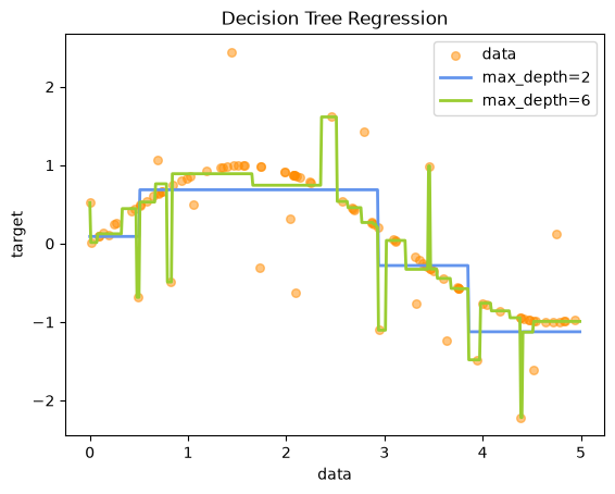

You can see that the model with max_depth=2 is underfitting, while the model with max_depth=6 is clearly overfitting. We can also evaluate the models with typical performance metrics such as $R^2$:

from sklearn.metrics import r2_score

r2_2 = r2_score(y_test, model1.predict(X_test))
r2_6 = r2_score(y_test, model2.predict(X_test))

print(f"R² (max_depth=2): {r2_2:.3f}")
print(f"R² (max_depth=6): {r2_6:.3f}")

R² (max_depth=2): 0.571
R² (max_depth=6): 0.472

Interactive: where does the tree stop helping?¶

Two depths make the point, but the full picture is more convincing. Drag the slider to grow the tree one level at a time and watch the step function chase the data:

import numpy as np
import plotly.graph_objects as go
import plotly.io as pio
from sklearn.metrics import r2_score

tpl = pio.templates["plotly_white"]
tpl.layout.paper_bgcolor = "rgba(0,0,0,0)"
tpl.layout.plot_bgcolor = "rgba(128,128,128,0.08)"
tpl.layout.font.color = "#888888"
pio.templates["psy300"] = tpl
pio.templates.default = "psy300"

depths = list(range(1, 13))
grid = np.arange(0.0, 5.0, 0.01)[:, np.newaxis]

traces, captions = [], []
for d in depths:
    tree = DecisionTreeRegressor(max_depth=d, random_state=0).fit(X_train, y_train)
    traces.append(go.Scatter(x=grid.ravel(), y=tree.predict(grid), mode="lines",
                             visible=False, line=dict(width=3, color="#55a868")))
    captions.append(
        f"max_depth = {d}   |   leaves = {tree.get_n_leaves()}   |   "
        f"train R² = {r2_score(y_train, tree.predict(X_train)):.3f}   |   "
        f"test R² = {r2_score(y_test, tree.predict(X_test)):.3f}"
    )
traces[0].visible = True

points = go.Scatter(x=X.ravel(), y=y, mode="markers", name="data",
                    marker=dict(size=8, color="darkorange", opacity=0.5))

slider_steps = []
for i, d in enumerate(depths):
    vis = [True] + [False] * len(traces)
    vis[i + 1] = True
    slider_steps.append(dict(method="update", label=str(d),
                             args=[{"visible": vis},
                                   {"annotations": [dict(x=0.5, y=1.12, xref="paper", yref="paper",
                                                         text=captions[i], showarrow=False,
                                                         font=dict(size=13), xanchor="center")]}]))

fig = go.Figure(data=[points] + traces)
fig.update_layout(
    sliders=[dict(active=0, currentvalue={"prefix": "Tree depth: "}, pad={"t": 40},
                  steps=slider_steps)],
    annotations=[dict(x=0.5, y=1.12, xref="paper", yref="paper", text=captions[0],
                      showarrow=False, font=dict(size=13), xanchor="center")],
    xaxis_title="data", yaxis_title="target", showlegend=False,
    margin=dict(l=10, r=10, t=80, b=20), height=480,
)
fig

The train R² keeps climbing towards 1 as the tree memorises individual points, while the test R² peaks early and then falls away. Note also how the number of leaves roughly doubles per level — a tree’s capacity grows exponentially in its depth, which is precisely why unrestricted trees overfit so readily.

The optimisation target¶

Regression trees choose splits to minimise within-node squared error. In the classical formulation, this is expressed as minimising the Residual Sum of Squares (RSS) across regions:

Finding the globally optimal partition into $J$ regions is often computationally infeasible. Instead, trees use recursive binary splitting:

• Top-down: start with all observations in a single region

• Greedy: at each step, choose the split that gives the largest immediate reduction in RSS

This means at each split, the algorithm selects:

• a single feature $X_k$, and

• a cutpoint $s$,

that minimise the RSS of the two resulting child nodes.

Note: In scikit-learn, the default criterion="squared_error" uses a variance/MSE-based impurity. This is equivalent to RSS because MSE is simply RSS scaled by the number of observations.

Learning break¶

Why can’t every possible kind of partition come from recursive binary splitting?

Classification Trees¶

Classification trees follow the same recursive splitting logic, but use different criteria to evaluate the splits, such as the classification error or purity measures. A popular purity measure is the Gini index, which is calculated as:

A small $G$ means high purity (mostly one class), while a large $G$ means low purity, indicating that a split does not separate the classes well. Here is an example with the Iris dataset, which contains measurements for three different types of iris flowers:

import matplotlib.pyplot as plt
from sklearn.tree import DecisionTreeClassifier, plot_tree
from sklearn.datasets import load_iris

# Load data
iris = load_iris()
X, y = iris.data, iris.target

clf = DecisionTreeClassifier(max_depth=3)
clf.fit(X, y)

plt.figure(figsize=(12,8))
plot_tree(clf, 
          feature_names=iris.feature_names,
          class_names=iris.target_names, 
          filled=True, rounded=True, fontsize=14);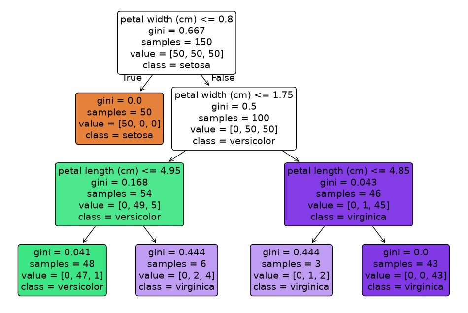

The tree plot of the fitted model contains the following information:

• Decision nodes

  • These are the rectangles with a splitting criterion (e.g. feature ≤ threshold)

  • They represent the points where the model splits the data and asks “which branch next?”

• Leaf nodes

  • The terminal rectangles without further splits

  • The leaf nodes mark the final predicted class (class)

• Color fill

  • The shade corresponds to the majority class at that node

  • The depth of color indicates purity (dark = almost all one class; light = mixture)

• Gini

  • Determines how pure a node is when choosing splits

  • The algorithm chooses splits that minimise weighted Gini impurity

• Tree depth

  • The number of levels indicates how many successive decisions are made

  • Capped by the max_depth parameter to control complexity

Another nice illustration is plotting the decision boundaries. As this works best with 2 features, we here showcase it for pairwise feature combinations:

Source

import numpy as np
from sklearn.inspection import DecisionBoundaryDisplay

# Plot settings
pairs      = [(0,1), (0,2), (0,3), (1,2), (1,3), (2,3)]
n_classes  = len(iris.target_names)
colors     = ["r", "g", "b"]
fig, axes  = plt.subplots(2, 3, figsize=(12, 8))
axes       = axes.ravel()

for ax, (i, j) in zip(axes, pairs):
    X_sub = X[:, [i, j]]
    clf = DecisionTreeClassifier(max_depth=4)
    clf.fit(X_sub, y)

    # Plot decision surface
    disp = DecisionBoundaryDisplay.from_estimator(
              clf, X_sub, cmap=plt.cm.RdYlBu, response_method="predict", 
              ax=ax, xlabel=iris.feature_names[i], ylabel=iris.feature_names[j])

    # Overlay training points
    for class_idx, color in zip(range(n_classes), colors):
        mask = (y == class_idx)
        ax.scatter(X_sub[mask, 0], X_sub[mask, 1], c=color, label=iris.target_names[class_idx], edgecolor="k", s=25)

    ax.set_title(f"{iris.feature_names[i]} vs {iris.feature_names[j]}")

# Legend and layout
handles, labels = axes[0].get_legend_handles_labels()
fig.legend(handles, labels, loc="lower center", ncol=n_classes, frameon=False)
fig.suptitle("Decision Surfaces")
plt.tight_layout();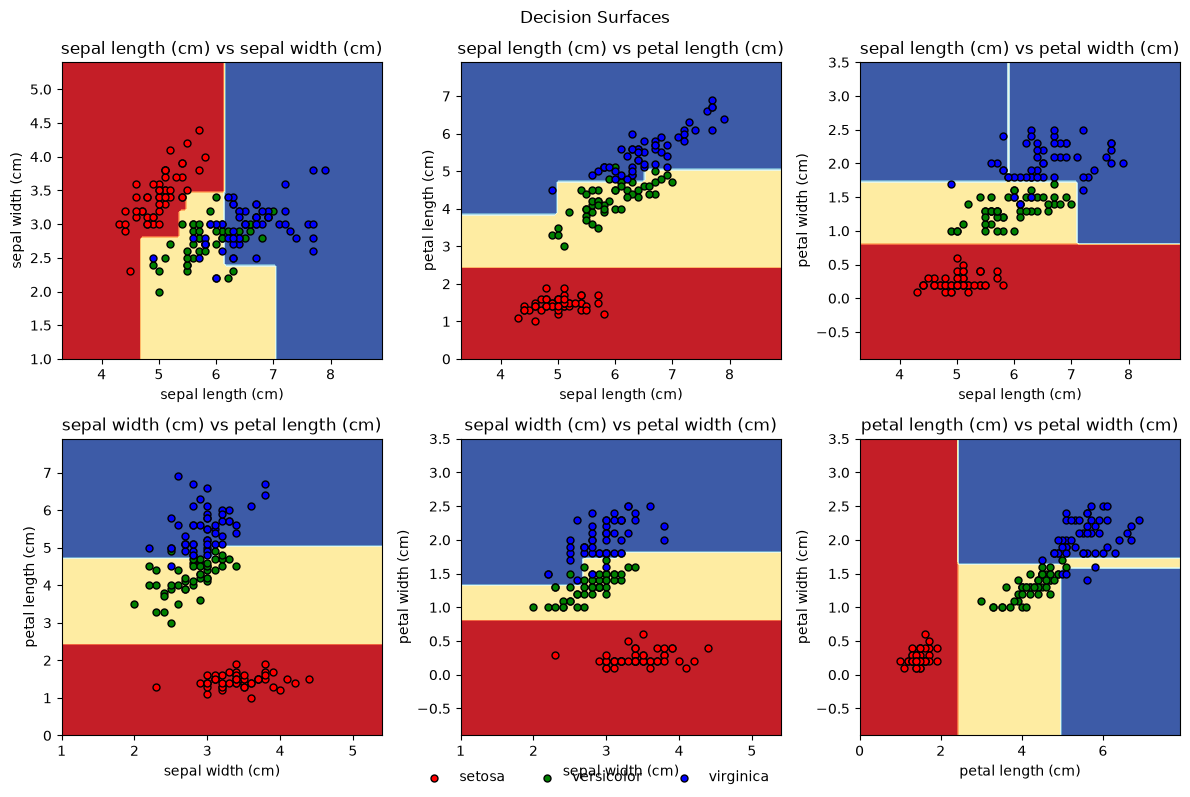

Overfitting and Pruning¶

Trees are vulnerable to overfitting. If allowed to grow without restriction, they become very deep and fit the training data extremely well. Such trees typically have low bias but high variance, leading to poor generalisation.

To counter this we can do multiple things:

• Prune the full-grown tree, also called bottom-up pruning or cost-complexity pruning (we saw this in the lecture)

• Tune the hyperparameters that control the tree-growing behavior, also called top-down pruning.

• Ensemble methods: bagging, random forests and boosting (will be introduced in the next sections)

Cost Complexity Pruning & Hyperparameter Tuning¶

Cost complexity pruning means we add a penalty for tree size such as:

$\text{Total Cost} = \text{RSS or Classification Error} + \alpha \cdot \text{Tree Size}$

In scikit-learn this is controlled by ccp_alpha

• ccp_alpha = 0 -> no pruning (full-grown tree)

• ccp_alpha > 0 -> pruning (smaller tree)

We can further control the tree growing behaviour with hyperparameters such as

• max_depth

• min_samples_split

• min_samples_leaf

We can use a grid search to find the best combination for some of these hyperparameters:

import numpy as np
from sklearn.tree import DecisionTreeClassifier
from sklearn.model_selection import GridSearchCV

iris = load_iris()
X, y = iris.data, iris.target
X_train, X_test, y_train, y_test = train_test_split(X, y, test_size=0.5, random_state=0)

param_grid = {
    'ccp_alpha':         np.linspace(0.0, 0.2, 10),
    'max_depth':         [2, 4, 6, 8, 10, None],
    'min_samples_split': [2, 5, 10, 20],
    'min_samples_leaf':  [1, 2, 4, 8],
}

grid = GridSearchCV(DecisionTreeClassifier(), param_grid, cv=5)
grid.fit(X_train, y_train)

print("Best params:", grid.best_params_)
print("Test set accuracy:", grid.score(X_test, y_test))

Best params: {'ccp_alpha': np.float64(0.0), 'max_depth': 4, 'min_samples_leaf': 1, 'min_samples_split': 2}
Test set accuracy: 0.96

Ensemble Methods¶

Single trees are prone to overfitting and generally are not competitive when compared to more sophisticated models such as support vector machines. Ensemble methods try to solve these issues by combining many trees to reduce variance (bagging, random forest) or bias (boosting).

Bagging (Bootstrap Aggregation)¶

Bagging aims to reduce variance by averaging many models trained on different bootstrap samples.

Suppose we train $B$ trees $T_1(x), \dots, T_B(x)$, each on its own bootstrap-resampled training set. At prediction time we combine them:

• Regression: take the arithmetic mean $\hat{f}_{\text{bag}}(x)=\frac{1}{B}\sum_{b=1}^{B} T_b(x)$.

• Classification: either average the class probabilities and choose the largest, or take a majority vote across the class labels predicted by the trees.

Because the trees are noisy but (approximately) unbiased, averaging drives down variance while leaving the expected prediction roughly unchanged. This is exactly the same intuition as averaging repeated noisy measurements of the same signal.

from sklearn.ensemble import BaggingClassifier
from sklearn.metrics import accuracy_score

bag = BaggingClassifier(n_estimators=200,
                        random_state=0,
                        oob_score=True)
bag.fit(X_train, y_train)
print("OOB score:", bag.oob_score_)

OOB score: 0.9466666666666667

Out-of-bag (OOB) score:

On average, about two-thirds of observations appear in any given bootstrap sample. The remaining one-third are out-of-bag (OOB) for that tree.

For each training observation, predictions are obtained only from trees for which that observation was OOB and then aggregated (majority vote for classification).

The OOB score reports the model’s performance on these OOB predictions. For classification, the default corresponds to the prediction accuracy, and with enough trees, the OOB score provides a strong internal estimate of test-set performance.

Random Forests¶

Random forests improve on bagging by decorrelating the trees. This is done by:

• Considering only a random subset of predictors at each split

• Drawing a fresh subset at every split

The final prediction still follows the same aggregation rules as bagging (average for regression, majority vote for classification). The extra randomness injected at each split makes the trees less correlated, so the averaging step cancels out even more variance than plain bagging.

from sklearn.ensemble import RandomForestClassifier

rf = RandomForestClassifier(n_estimators=100, random_state=0)
rf.fit(X_train, y_train)

accuracy_score(y_test, rf.predict(X_test))

The impurity-based feature importance can be visualised as:

import seaborn as sns

sns.barplot(x=rf.feature_importances_, y=iris.feature_names)
plt.title("Feature Importance");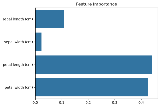

Boosting¶

Boosting is an ensemble strategy that builds models sequentially, where each new tree focuses on correcting the errors made by the previous ones. In contrast to bagging and random forests, boosting does not train trees independently.

The core idea is to combine many weak learners (typically shallow trees) into a single strong predictive model:

1. Fit a simple tree to the data

2. Identify observations that are predicted poorly

3. Increase the influence (weight) of these observations

4. Fit a new tree that focuses more on the difficult cases

5. Repeat and combine all trees

Each individual tree is usually very small (often depth 1-3) and only slightly better than random guessing. The strength of boosting comes from accumulating many such small improvements. If we denote the $m$-th tree by $T_m(x)$ and its fitted weight by $\gamma_m$, the boosted prediction after $M$ trees is typically

where $F_0$ is the constant initial prediction and the learning rate $\eta$ shrinks each tree’s contribution. Because the trees are added sequentially, later trees are trained on the residuals (or gradient directions) left unexplained by the earlier ones.

Boosted trees involve several interacting hyperparameters:

• Number of trees: more trees increase model capacity

• Tree depth: shallow trees reduce variance and overfitting

• Learning rate $\eta$: controls how strongly each tree contributes

A common rule of thumb is to use a small learning rate and to compensate with more trees:

from sklearn.ensemble import GradientBoostingClassifier

boost = GradientBoostingClassifier(n_estimators=200,
                                   learning_rate=0.05,
                                   max_depth=2,
                                   random_state=42)
boost.fit(X_train, y_train)

accuracy_score(y_test, boost.predict(X_test))

Advantages

• Often achieves very high predictive accuracy

• Can model complex non-linear relationships

• Strong performance using relatively small trees

Disadvantages

• Sensitive to hyperparameter choices

• Can overfit if trees are too deep or learning rate too large

• Less interpretable than single trees

Summary¶