〰️ Polynomial and Flexible Regression - Statistical Learning with Python

Let us have a quick recap of the first session of the semester, where regression models were introduced. In linear regression, we assume that the relationship between a predictor $x$ and a response $y$ is a straight line:

y \approx \beta_0 + \beta_1 x.

(1)

In many real-world problems, this assumption is too restrictive. The true relationship may be curved, bend differently in different regions of $x$ , or vary smoothly but non-linearly.

In this chapter, we look at four families of methods that allow more flexible regression functions:

Polynomial regression
Stepwise regression
Spline regression
Local regression

Let’s start by creating some example data. Imagine we have one predictor $x$ and a response $y$ generated as:

y = \sin(x) + \varepsilon, \quad \varepsilon \sim \mathcal{N}(0, \sigma^2).

(2)

import numpy as np
import pandas as pd
import matplotlib.pyplot as plt

rng = np.random.default_rng(42)

n = 200
X = np.linspace(0, 10, n)
eps = rng.normal(scale=0.4, size=n)
y = np.sin(X) + 0.3 * X + eps
data = pd.DataFrame({"x": X, "y": y})

fig, ax = plt.subplots()
ax.scatter(data["x"], data["y"], alpha=0.5)
ax.set(xlabel="x", ylabel="y");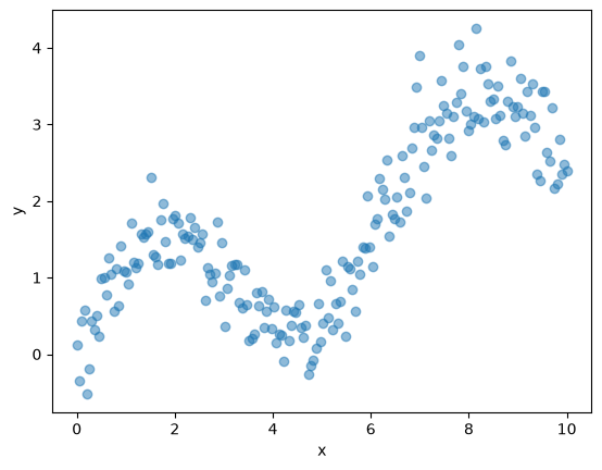

If we fit a straight line to such data, the model will clearly miss the oscillating pattern. Flexible regression methods aim to recover such non-linear patterns while still being based on the same least squares framework.

Polynomial Regression¶

Polynomial regression extends the linear model by including powers of $x$ as additional predictors:

Degree 1 (ordinary linear regression):
$y \approx \beta_0 + \beta_1 x$
(3)
Degree 2 (quadratic):
$y \approx \beta_0 + \beta_1 x + \beta_2 x^2$
(4)
Degree $d$ :
$y \approx \beta_0 + \beta_1 x + \beta_2 x^2 + \dots + \beta_d x^d.$
(5)

Pros:

Simple and easy to fit with ordinary least squares
Can capture smooth non-linear trends with low-degree polynomials

Cons:

High-degree polynomials can oscillate wildly (especially at the boundaries)
Global basis: changing the fit in one region can affect the entire curve

We can conveniently generate polynomial features using PolynomialFeatures from sklearn.preprocessing and then fit a standard LinearRegression model.

from sklearn.preprocessing import PolynomialFeatures
from sklearn.linear_model import LinearRegression

def fit_poly_regression(x, y, degree):
    """Fit a polynomial regression of given degree and return the model + grid predictions."""
    x = np.asarray(x).reshape(-1, 1)
    poly = PolynomialFeatures(degree=degree, include_bias=False)
    X_poly = poly.fit_transform(x)

    model = LinearRegression()
    model.fit(X_poly, y)

    # For visualisation: predictions on a dense grid
    x_grid = np.linspace(x.min(), x.max(), 300).reshape(-1, 1)
    X_grid_poly = poly.transform(x_grid)
    y_hat = model.predict(X_grid_poly)

    return model, x_grid.ravel(), y_hat

degrees = [1, 2, 4, 16]

fig, ax = plt.subplots()
ax.scatter(data["x"], data["y"], alpha=0.3, label="Data")

for d in degrees:
    _, xg, yg = fit_poly_regression(data["x"], data["y"], degree=d)
    ax.plot(xg, yg, label=f"Degree {d}")
ax.set(xlabel="x", ylabel="y", title="Polynomial regression with different degrees")
plt.legend();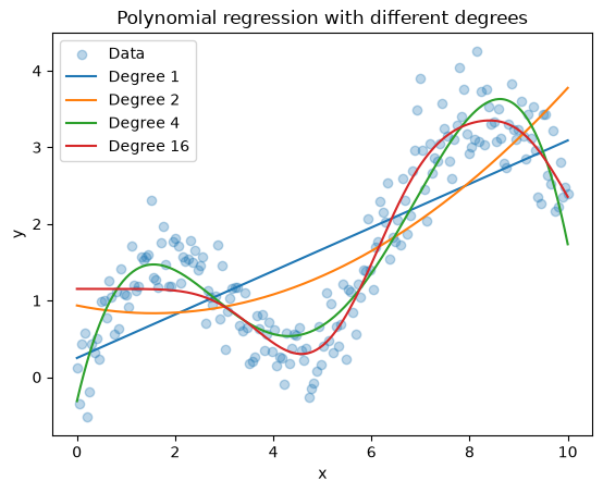

Things to observe:

Degree 1 (straight line) cannot follow the curvature.
Degree 2 or 3 often works well for gently curved relationships.
Higher degree models can start to wiggle and overfit the noise.

Piecewise Constant Regression¶

The simple idea:

Divide the range of $x$ into intervals using cut points (knots) and fit a constant mean within each interval.

Concretely, choose cut points $c_1 < c_2 < \dots < c_K$ and define indicator variables

I_1(x) = \mathbf{1}(x \le c_1), \quad I_2(x) = \mathbf{1}(c_1 < x \le c_2), \dots, I_{K+1}(x) = \mathbf{1}(x > c_K).

(6)

Then the model is

y \approx \beta_0 + \beta_1 I_1(x) + \dots + \beta_{K+1} I_{K+1}(x),

(7)

which produces a piecewise constant (stepwise) regression function. This is equivalent to a B-spline of degree 0 (a “zero-order spline”).

Pros:

Very simple and interpretable: one mean per age/x-interval
Useful as a starting point to understand more flexible splines

Cons:

The fit is discontinuous at the cut points
Sensitive to the choice and placement of cut points
Can look rough; higher-order splines often give smoother fits

We can build a 0th-order spline (step function) basis using patsy.dmatrix with bs(..., degree=0) and then fit a linear model with statsmodels:

import patsy
import statsmodels.api as sm

# Choose some cut points (knots) over the x-range
cut_points = (2, 4, 6, 8)

# Build a B-spline basis of degree 0 (step function)
transformed_x = patsy.dmatrix(
    "bs(x, knots=cut_points, degree=0, include_intercept=False)",
    {"x": data["x"], "cut_points": cut_points},
    return_type="dataframe",
)

Fit the model:

step_model = sm.OLS(data["y"], transformed_x)
step_fit = step_model.fit()

print(step_fit.summary())

                            OLS Regression Results                            
==============================================================================
Dep. Variable:                      y   R-squared:                       0.757
Model:                            OLS   Adj. R-squared:                  0.752
Method:                 Least Squares   F-statistic:                     152.2
Date:                Wed, 12 Aug 2026   Prob (F-statistic):           8.05e-59
Time:                        14:16:17   Log-Likelihood:                -167.85
No. Observations:                 200   AIC:                             345.7
Df Residuals:                     195   BIC:                             362.2
Df Model:                           4                                         
Covariance Type:            nonrobust                                         
=================================================================================================================================
                                                                    coef    std err          t      P>|t|      [0.025      0.975]
---------------------------------------------------------------------------------------------------------------------------------
Intercept                                                         1.0069      0.090     11.227      0.000       0.830       1.184
bs(x, knots=cut_points, degree=0, include_intercept=False)[0]     0.0223      0.127      0.176      0.861      -0.228       0.272
bs(x, knots=cut_points, degree=0, include_intercept=False)[1]    -0.4055      0.127     -3.197      0.002      -0.656      -0.155
bs(x, knots=cut_points, degree=0, include_intercept=False)[2]     1.6288      0.127     12.843      0.000       1.379       1.879
bs(x, knots=cut_points, degree=0, include_intercept=False)[3]     2.0670      0.127     16.297      0.000       1.817       2.317
==============================================================================
Omnibus:                        0.227   Durbin-Watson:                   0.792
Prob(Omnibus):                  0.893   Jarque-Bera (JB):                0.357
Skew:                          -0.062   Prob(JB):                        0.837
Kurtosis:                       2.834   Cond. No.                         5.83
==============================================================================

Notes:
[1] Standard Errors assume that the covariance matrix of the errors is correctly specified.

Visualise the stepwise fit:

xp = np.linspace(data["x"].min(), data["x"].max(), 300)
xp_trans = patsy.dmatrix(
    "bs(xp, knots=cut_points, degree=0, include_intercept=False)",
    {"xp": xp, "cut_points": cut_points},
    return_type="dataframe",
)

pred_step = step_fit.predict(xp_trans)

plt.figure(figsize=(10, 6))
plt.scatter(data["x"], data["y"], alpha=0.4, label="Data")
plt.plot(xp, pred_step, color="red", label="Stepwise fit (degree 0)")
for c in cut_points:
    plt.axvline(c, color="black", linestyle="--", alpha=0.6)

plt.xlabel("x")
plt.ylabel("y")
plt.title("Stepwise regression (zero-order spline)")
plt.legend();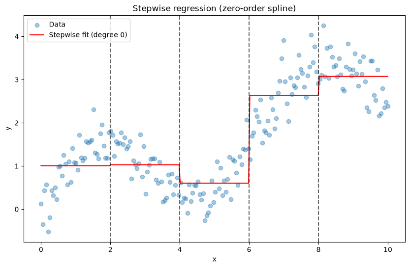

Spline Regression¶

The previous section introduced “stepwise regression” as 0th-order splines. However, when we talk about spline regression, we usually mean higher-order splines, which will smooth these steps into continuous and differentiable curves. Again, the key idea is the similar:

Approximate the regression function by piecewise polynomials that are smoothly joined at pre-defined points called knots.

For example, a cubic spline with knots at $t_1, \dots, t_K$ is a function that is:

A cubic polynomial on each interval $(-\infty, t_1)$ , $(t_1, t_2)$ , …, $(t_K, \infty)$
Continuously differentiable up to a certain order at the knots

We usually do not work with the piecewise form directly. Instead, we represent splines as a linear combination of basis functions:

f(x) = \sum_{j=1}^{M} \theta_j B_j(x),

(8)

where $B_j(x)$ are spline basis functions (B-splines). This again gives a linear model in the parameters $\theta_j$ .

Two common options:

B-splines (flexible general basis)
Natural splines (add boundary constraints to avoid wild extrapolation)

Again, we use the convenient bs() function from patsy to create B-spline bases. We can then plug these into statsmodels for ordinary least squares:

from patsy import dmatrix

# Build a cubic B-spline basis with 6 degrees of freedom
spline_basis = dmatrix(
    "bs(x, df=6, degree=3, include_intercept=False)",
    {"x": data["x"]},
    return_type="dataframe",
)

Fit an OLS model:

spline_model = sm.OLS(data["y"], spline_basis).fit()
print(spline_model.summary())

                            OLS Regression Results                            
==============================================================================
Dep. Variable:                      y   R-squared:                       0.906
Model:                            OLS   Adj. R-squared:                  0.903
Method:                 Least Squares   F-statistic:                     308.2
Date:                Wed, 12 Aug 2026   Prob (F-statistic):           5.30e-96
Time:                        14:16:17   Log-Likelihood:                -73.555
No. Observations:                 200   AIC:                             161.1
Df Residuals:                     193   BIC:                             184.2
Df Model:                           6                                         
Covariance Type:            nonrobust                                         
=====================================================================================================================
                                                        coef    std err          t      P>|t|      [0.025      0.975]
---------------------------------------------------------------------------------------------------------------------
Intercept                                            -0.2490      0.155     -1.604      0.110      -0.555       0.057
bs(x, df=6, degree=3, include_intercept=False)[0]     1.8920      0.290      6.527      0.000       1.320       2.464
bs(x, df=6, degree=3, include_intercept=False)[1]     2.0838      0.189     11.049      0.000       1.712       2.456
bs(x, df=6, degree=3, include_intercept=False)[2]    -0.6812      0.231     -2.947      0.004      -1.137      -0.225
bs(x, df=6, degree=3, include_intercept=False)[3]     4.6825      0.214     21.838      0.000       4.260       5.105
bs(x, df=6, degree=3, include_intercept=False)[4]     3.3392      0.241     13.834      0.000       2.863       3.815
bs(x, df=6, degree=3, include_intercept=False)[5]     2.7045      0.216     12.516      0.000       2.278       3.131
==============================================================================
Omnibus:                        2.725   Durbin-Watson:                   1.790
Prob(Omnibus):                  0.256   Jarque-Bera (JB):                2.671
Skew:                           0.281   Prob(JB):                        0.263
Kurtosis:                       2.933   Cond. No.                         19.7
==============================================================================

Notes:
[1] Standard Errors assume that the covariance matrix of the errors is correctly specified.

Visualise the spline fit:

x_grid = np.linspace(data["x"].min(), data["x"].max(), 300)
spline_grid = dmatrix(
    "bs(x, df=6, degree=3, include_intercept=False)",
    {"x": x_grid},
    return_type="dataframe",
)
y_spline_hat = spline_model.predict(spline_grid)

fig, ax = plt.subplots()
ax.scatter(data["x"], data["y"], alpha=0.3, label="Data")
ax.plot(x_grid, y_spline_hat, label="Cubic B-spline (df = 6)", linewidth=2)
ax.set_xlabel("x")
ax.set_ylabel("y")
ax.set_title("Spline regression")
ax.legend();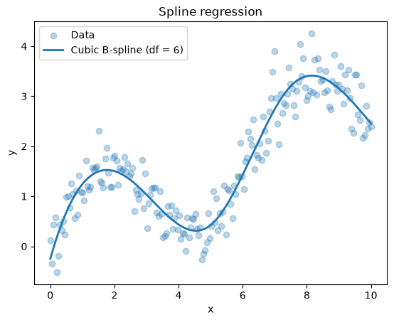

Local Regression (LOWESS)¶

Polynomial and spline regression still use a global basis: one set of parameters applies to the whole range of $x$ . Local regression takes a different view:

Fit a separate regression in a neighbourhood around each target point, using only nearby observations (with weights).

For a target point $x_0$ :

Define a neighbourhood around $x_0$ , e.g. the closest $\alpha \cdot n$ observations, where $\alpha$ is a smoothing parameter between 0 and 1.
Assign weights to observations, typically higher for points closer to $x_0$ .
Fit a weighted least squares regression (often linear or quadratic) using those weighted points.
The fitted value at $x_0$ is the prediction from this local model.

Repeat this for many $x_0$ to obtain a smooth curve.

Key parameters:

Span / fraction (frac): proportion of data used in each local fit
- Small frac → very flexible, risk of overfitting
- Large frac → smoother, less flexible
Degree of local polynomial (often 1 or 2)

statsmodels provides a convenient implementation of LOWESS (locally weighted scatterplot smoothing).

from statsmodels.nonparametric.smoothers_lowess import lowess

x = data["x"].to_numpy()
y = data["y"].to_numpy()

# Try different fractions
frac_list = [0.2, 0.5, 0.7]

fig, ax = plt.subplots()
ax.scatter(x, y, alpha=0.3, label="Data")

for frac in frac_list:
  result = lowess(y, x, frac=frac, return_sorted=True)
  ax.plot(result[:, 0], result[:, 1], label=f"LOWESS, frac = {frac}", linewidth=2)

ax.set(xlabel="x", ylabel="y", title="Local regression (LOWESS) with different spans")
ax.legend();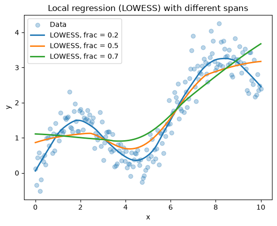

Observe:

frac = 0.2 follows the data more closely (more wiggles).
frac > 0.5 gives a more general trend.

Local regression methods are very useful for exploratory analysis: they give a flexible, data-driven summary of the trend without a strong global parametric assumption.

Interactive: how much flexibility is too much?¶

All four methods have exactly one knob that controls flexibility — the polynomial degree, the number of cut points, the spline degrees of freedom, and the LOWESS span. Below you can turn that knob for each method and watch the fit respond. The reported errors come from a 70/30 train/test split, so you can also see where the extra flexibility stops paying off.

import numpy as np
import plotly.graph_objects as go
import plotly.io as pio
from patsy import dmatrix
from sklearn.model_selection import train_test_split
from sklearn.metrics import mean_squared_error
from statsmodels.nonparametric.smoothers_lowess import lowess
import statsmodels.api as sm

tpl = pio.templates["plotly_white"]
tpl.layout.paper_bgcolor = "rgba(0,0,0,0)"
tpl.layout.plot_bgcolor = "rgba(128,128,128,0.08)"
tpl.layout.font.color = "#888888"
pio.templates["psy300"] = tpl
pio.templates.default = "psy300"

x_all = data["x"].to_numpy()
y_all = data["y"].to_numpy()
x_tr, x_te, y_tr, y_te = train_test_split(x_all, y_all, test_size=0.3, random_state=0)
grid = np.linspace(x_all.min(), x_all.max(), 300)


def fit_predict(method, setting):
    """Return (grid predictions, train MSE, test MSE) for one method/setting."""
    if method == "poly":
        c = np.polyfit(x_tr, y_tr, setting)
        return np.polyval(c, grid), np.polyval(c, x_tr), np.polyval(c, x_te)

    if method in ("step", "spline"):
        degree = 0 if method == "step" else 3
        formula = f"bs(v, df={setting}, degree={degree}, include_intercept=True)"
        basis_tr = dmatrix(formula, {"v": x_tr}, return_type="dataframe")
        model = sm.OLS(y_tr, basis_tr).fit()
        pred = lambda v: model.predict(
            dmatrix(basis_tr.design_info, {"v": v}, return_type="dataframe"))
        return pred(grid), pred(x_tr), pred(x_te)

    # LOWESS has no parametric form, so we interpolate its fitted curve
    sm_fit = lowess(y_tr, x_tr, frac=setting, return_sorted=True)
    pred = lambda v: np.interp(v, sm_fit[:, 0], sm_fit[:, 1])
    return pred(grid), pred(x_tr), pred(x_te)


configs = [
    ("poly",   "Polynomial degree",  "poly", [1, 2, 3, 5, 8, 12, 18]),
    ("step",   "Step function (df)", "step", [2, 3, 4, 6, 8, 12, 20]),
    ("spline", "Cubic spline (df)",  "spl",  [4, 5, 6, 8, 10, 15, 25]),
    ("lowess", "LOWESS span (frac)", "low",  [0.1, 0.2, 0.3, 0.5, 0.7, 0.9]),
]

traces, steps = [], []
for method, label, tag, settings in configs:
    for s in settings:
        y_grid, y_hat_tr, y_hat_te = fit_predict(method, s)
        traces.append(go.Scatter(x=grid, y=y_grid, mode="lines", visible=False,
                                 line=dict(width=3, color="#c44e52"),
                                 name=f"{label} = {s}"))
        steps.append((label, s, f"{tag} {s:g}",
                      mean_squared_error(y_tr, y_hat_tr),
                      mean_squared_error(y_te, y_hat_te)))

scatter = go.Scatter(x=x_all, y=y_all, mode="markers", name="Data",
                     marker=dict(size=6, color="lightgrey",
                                 line=dict(color="gray", width=1)))
traces[0].visible = True


def caption(i):
    label, s, _, mtr, mte = steps[i]
    return f"{label} = {s:g}   |   train MSE = {mtr:.3f}   |   test MSE = {mte:.3f}"


slider_steps = []
for i in range(len(traces)):
    vis = [True] + [False] * len(traces)
    vis[i + 1] = True
    slider_steps.append(dict(
        method="update", label=steps[i][2],
        args=[{"visible": vis},
              {"annotations": [dict(x=0.5, y=1.12, xref="paper", yref="paper",
                                    text=caption(i), showarrow=False,
                                    font=dict(size=13), xanchor="center")]}]))

fig = go.Figure(data=[scatter] + traces)
fig.update_layout(
    sliders=[dict(active=0, currentvalue={"prefix": "Flexibility setting: "},
                  font=dict(size=10), pad={"t": 40}, steps=slider_steps)],
    annotations=[dict(x=0.5, y=1.12, xref="paper", yref="paper", text=caption(0),
                      showarrow=False, font=dict(size=13), xanchor="center")],
    xaxis_title="x", yaxis_title="y", showlegend=False,
    margin=dict(l=10, r=10, t=80, b=20), height=500,
)
fig

The slider walks through all four method families in turn (polynomial, then steps, then splines, then LOWESS). Watch the two error numbers as you drag: the train MSE decreases monotonically for every method, while the test MSE bottoms out and then climbs. That gap is the bias-variance tradeoff of ⚖️ Bias-Variance Tradeoff, now visible for four different notions of “flexibility”.

Summary and Quiz¶

Method	Key Idea	Flexibility	Pros	Cons
Polynomial Regression	Powers of $x$ as predictors: $x, x^2, \dots, x^d$	Controlled by degree $d$	Simple to fit with OLS; interpretable	Oscillates at boundaries; global changes affect entire curve
Piecewise Constant Regression	Constant values in intervals defined by knots	Controlled by knots	Simple and interpretable	Discontinuous at knots; sensitive to knot placement
Spline Regression	Piecewise polynomials smoothly joined at knots	Controlled by knots and degree	Smooth and flexible; mostly local	Requires choosing knots; can overfit with many knots
Local Regression (LOWESS)	Weighted regression in neighborhood of each point	Controlled by span/fraction	Data-driven; no global assumptions	Computationally intensive; requires choosing span; harder to interpret

In the lecture, all methods except simple polynomial regression are considered local models. In piecewise constant regression, only the information within each bin contributes to the fitted value in that region. Spline regression is also largely local, but neighbouring intervals are coupled through smoothness constraints at the knots, which introduces a limited amount of global structure.

In practice, these methods are often combined with regularisation and cross-validation to control overfitting and to select tuning parameters such as the degree, number and location of knots, or the span.