📈 From AdaBoost to Gradient Boosting - Statistical Learning with Python

As we explored in the previous session, boosting refers to a class of ensemble methods that build predictive models sequentially, where each new model focuses on the errors made by previous ones. Historically, boosting was first introduced for classification in the form of AdaBoost. The same core idea can be extended to regression and leads naturally to gradient boosting, which is the main focus of this session.

This notebook therefore serves two purposes:

Use AdaBoost for regression as an intuitive starting point
Transition to gradient boosting for regression as the principled and modern formulation

Intuition: Weak regressors can form strong predictors¶

Suppose we have a regression problem with inputs $x_i$ and continuous targets $y_i$ .

A weak regressor is a model that performs only slightly better than a very naive baseline, such as predicting the mean of the target variable. On its own, such a model is not very useful. However, many weak regressors combined carefully can yield a strong predictive model.

The basic boosting idea is:

Fit a simple model to the data
Identify where this model performs poorly
Encourage the next model to focus on these difficult observations
Combine all models into a single predictor

AdaBoost for regression¶

AdaBoost implements this idea by assigning weights to observations. Observations that are predicted poorly receive larger weights and therefore influence the next model more strongly.

We observe training data

\{(x_i, y_i)\}_{i=1}^N

(1)

and maintain observation weights

w_i^{(m)}

(2)

which change after each boosting iteration $m$ . Initially, all observations are weighted equally:

w_i^{(1)} = \frac{1}{N}

(3)

Choice of weak learner

In regression settings, AdaBoost typically relies on very simple base learners, such as

decision stumps (trees with depth one)
very shallow regression trees

The goal is not to fit the data well in a single step, but to make small, incremental improvements.

Measuring regression error

For regression, misclassification counts are no longer meaningful. Instead, prediction errors are measured using absolute deviations:

e_i = |y_i - \hat{y}_i|

(4)

To make errors comparable across observations, they are normalised:

L_i = \frac{e_i}{\max_j e_j}

(5)

so that $0 \le L_i \le 1$ . Observations with larger errors receive stronger penalties.

The AdaBoost.R2 algorithm¶

For boosting rounds $m = 1, \dots, M$ :

Fit a weak regressor $T_m(x)$ using the current weights $w_i^{(m)}$
Compute normalised errors $L_i$
Compute the weighted error rate

\text{err}_m = \sum_{i=1}^N w_i^{(m)} L_i

(6)

Compute the model weight

\alpha_m = \log\left(\frac{1 - \text{err}_m}{\text{err}_m}\right)

(7)

Update observation weights

w_i^{(m+1)} = w_i^{(m)} \cdot \exp(\alpha_m L_i)

(8)

Renormalise the weights so that they sum to one

Observations with large errors gain influence over subsequent regressors.

Final prediction

The final AdaBoost regression model is a weighted sum of weak regressors:

\hat{f}(x) = \sum_{m=1}^M \alpha_m T_m(x)

(9)

Each regressor contributes according to its predictive performance.

Limitations¶

While AdaBoost captures the idea of sequential error correction, it has several limitations in regression problems:

the definition and normalisation of errors is somewhat ad hoc
the method is sensitive to outliers
there is no explicit loss function being minimised
the optimisation perspective remains unclear

These limitations motivate a more principled approach to boosting.

From AdaBoost to gradient boosting¶

Gradient boosting reformulates boosting as an explicit optimisation problem. Instead of reweighting observations, it constructs models that directly minimise a chosen loss function.

The key idea is to view boosting as gradient descent in function space.

Core idea¶

Start with a simple initial model, usually the mean of the target values
Compute residuals between observed targets and current predictions
Fit a small regression tree to these residuals
Add this tree to the model, scaled by a learning rate
Repeat

Each new tree explains structure that previous trees failed to capture.

After $M$ iterations, the model can be written as

\hat{F}_M(x) = F_0 + \sum_{m=1}^M \eta \, T_m(x)

(10)

where $F_0$ is the constant starting model (the mean of $y$ ) and $\eta$ denotes the learning rate.

Gradient boosting offers several advantages. It:

works naturally for regression problems
allows arbitrary differentiable loss functions
is less sensitive to outliers than AdaBoost
forms the basis of modern methods such as XGBoost and LightGBM

For these reasons, gradient boosting has largely replaced AdaBoost in regression settings.

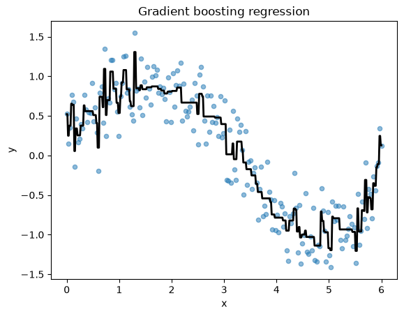
Example¶

import numpy as np
import matplotlib.pyplot as plt
from sklearn.ensemble import GradientBoostingRegressor

rng = np.random.RandomState(0)
X = np.linspace(0, 6, 200).reshape(-1,1)
y = np.sin(X).ravel() + rng.normal(scale=0.3, size=200)

gb = GradientBoostingRegressor(
      n_estimators=200,
      learning_rate=0.1,
      max_depth=2,
      random_state=0)
gb.fit(X, y)

X_plot = np.linspace(0, 6, 500).reshape(-1,1)
y_pred = gb.predict(X_plot)

fig, ax = plt.subplots()
ax.scatter(X, y, s=20, alpha=0.5)
ax.plot(X_plot, y_pred, color="black", linewidth=2)
ax.set(title="Gradient boosting regression", xlabel="x", ylabel="y");