📊 Logistic Regression - Statistical Learning with Python

Before applying logistic regression to model our data, we will attempt to do so through simple linear regression. While linear regression is not suitable for dichotomous outcomes, visualizing it can help illustrate why logistic regression is a better fit for our research question.

Why Not Linear Regression?¶

import pandas as pd
import seaborn as sns
import matplotlib.pyplot as plt

df = pd.read_csv("data.dat", delimiter='\t')

fig, ax = plt.subplots()
sns.regplot(x="age", y="display", data=df, ax=ax)
ax.set(xlabel="Age [month]", ylabel="Understanding display rules")

plt.show()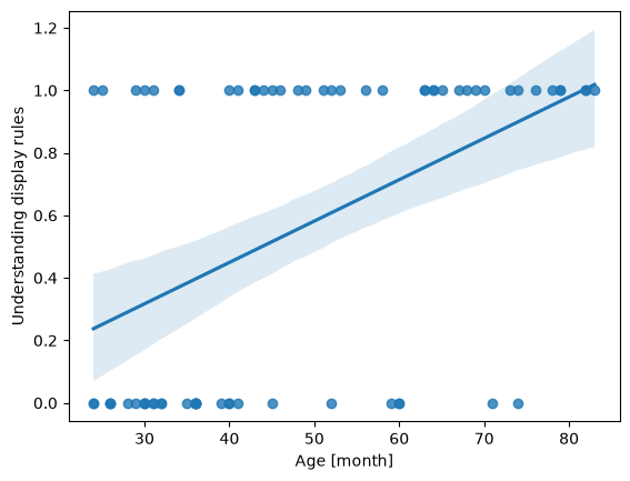

Linear regression assumes that the dependent variable is continuous and unbounded. When we apply it to a dichotomous outcome such as understanding display rules (0/1), the underlying assumptions break down:

The model can produce predicted values <0 or >1, which are impossible probabilities.
Linear regression assumes homoscedasticity (constant variance of errors), which binary data violate by construction.

Logistic Regression with Python¶

In this example, we will use the LogisticRegression() class from scikit-learn for modeling.

import numpy as np
from sklearn.linear_model import LogisticRegression

# Convert 'age' into a NumPy array and reshape it to a 2D array (required for the model)
# .reshape(-1, 1): Creates one column with as many rows as needed (-1 infers the row count)
X = np.asarray(df['age']).reshape(-1, 1)

# Convert 'display' to a NumPy array for the binary outcome
y = np.asarray(df['display']) # binary outcome

model = LogisticRegression()
results = model.fit(X, y)

print(f"Intercept: {results.intercept_}")
print(f"Coefficients: {results.coef_}")

Intercept: [-2.83306013]
Coefficients: [[0.06612023]]

Interpreting the Model Outputs: Logits¶

The logistic regression still gives us an intercept and a slope, but they operate on the log-odds scale, not the probability scale:

Intercept: The expected logit (log-odds) of the outcome (understanding display rules) when age = 0.
Slope/coefficient: The logit increase of understanding display rules for each one-month increase in age.

This means the output of a logistic regression model is linear in the log-odds (logits). Each coefficient in the logistic regression tells us how a one-unit change in a predictor affects the log-odds of the outcome. While not as intuitive as probabilities, the transformation to logits is crucial because it allows us to use linear regression techniques for binary outcomes.

But what even are logits?

Logits are the natural logarithm of the odds of an event occurring in logistic regression. The odds of an event are defined as the ratio of the probability of the event occurring ( $P$ ) to the probability of the event not occurring $(1-P)$ :

\text{Odds} = \frac{P}{1-P}

(1)

In logistic regression, we predict the logit (log-odds) as a linear combination of the independent variables $(X_1, X_2, \dots, X_k)$ and their corresponding regression coefficients $(\beta_1, \beta_2, \dots \beta_k)$ :

\text{Logit}(P) = \ln\left(\frac{P}{1-P}\right) = \beta_0 + \beta_1X_1 + \beta_2X_2 + \dots + \beta_kX_k

(2)

If we plot the equation, we can see how the regression line looks like:

df['logit'] = results.intercept_ + results.coef_[0] * df['age']

fig, ax = plt.subplots()
ax.plot(df['age'], df['logit'], color="red", label="Logit Transform")
ax.scatter(df['age'], df['logit'], color="blue", alpha=0.5, label="Data points")
ax.set(xlabel="Age", ylabel="Logit (Log-Odds)", title="Logit Transform")

plt.legend()
plt.show()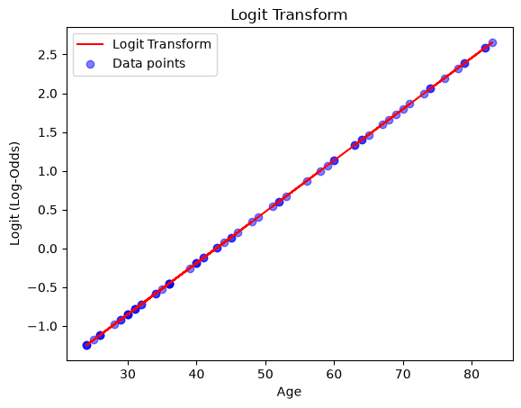

From Logits to Probabilities¶

We can simply transform the logits back into probabilities (more specifically the conditional probability of an observation $y$ belonging to class 1 given predictor(s) $X$ ):

P(Y=1 \mid X) = \frac{1}{1 + e^{-(b_0 + b_1 X)}}

(3)

To better understand the model’s behavior, let’s plot its outputs. A simple way to do this is by creating an evenly spaced array of values for our range, and then use model.predict_proba() to predict the outcome for each value. This will generate the regression line:

# Create an evenly spaced array of values for the range 
x_range = np.linspace(1, 100, 100).reshape(-1, 1) 

# Predict probability of class 1 for each value in the range
y_prob = model.predict_proba(x_range)
y_prob = y_prob[:,1] # only get the second column

# Plot the results
fig, ax = plt.subplots()
ax.scatter(X, y, color='blue', label='data points', alpha=0.5)   # actual data
ax.plot(x_range, y_prob, color='red', label='model predictions') # regression model
ax.set(xlabel='age', ylabel='display', title='Logistic Regression Model')

plt.legend()
plt.show()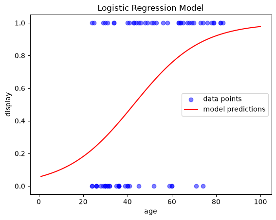

Model Evaluation¶

To evaluate our model, we can examine how many values of $y$ (understanding display rules) were predicted correctly by the model. For this, we could binarise the probabilities as returned from model.predict_proba() or we can also just simply use model.predict():

import numpy as np
import pandas as pd
import seaborn as sns
import matplotlib.pyplot as plt
from sklearn.linear_model import LogisticRegression

df = pd.read_csv("data.dat", delimiter='\t')
X = np.asarray(df['age']).reshape(-1, 1) 
y = np.asarray(df['display'])

model = LogisticRegression()
results = model.fit(X, y)

predictions = model.predict(X)
accuracy =  model.score(X, y)

print("Model predictions:", predictions)
print("\nAccuracy:", accuracy)

Model predictions: [0 0 0 0 0 0 0 0 0 0 0 0 0 0 0 0 0 0 0 0 0 0 0 0 1 0 0 0 1 0 0 0 1 1 1 0 0
 1 1 0 1 1 1 1 1 1 1 1 1 1 1 1 1 1 1 1 1 1 1 1 1 1 1 1 1 1 1 1 1 1]

Accuracy: 0.7714285714285715

An accuracy of 77% indicates the that the model correctly predicts the outcome for about 77% of the children in our data. This suggests that the model performs reasonably well, although it still misclassifies some cases. For a more detailed investigation, a confusion matrix is a useful way to visualize the prediction accuracy:

from sklearn.metrics import confusion_matrix, classification_report
print(f"Confusion matrix:\n {confusion_matrix(y, model.predict(X))}")

Confusion matrix:
 [[24  7]
 [ 9 30]]

The output of the confusion matrix provides the following values:

	Predicted Negative	Predicted Positive
Actual Negative	True Negative (TN)	False Positive (FP)
Actual Positive	False Negative (FN)	True Positive (TP)

For an even deeper inspection of the model’s accuracy, we can print the classification report:

report = classification_report(y, model.predict(X))
print(report)

              precision    recall  f1-score   support

           0       0.73      0.77      0.75        31
           1       0.81      0.77      0.79        39

    accuracy                           0.77        70
   macro avg       0.77      0.77      0.77        70
weighted avg       0.77      0.77      0.77        70

The output can be interpreted as follows:

Precision: Proportion of correct predictions among all predictions for that class.

\text{Precision} = \frac{\text{True Positives (TP)}}{\text{True Positives (TP)} + \text{False Positives (FP)}}

(4)

Class 0: when the model predicts that a sample does not understand the display rules (Class 0), 73% of the time it is correct.
Class 1: when the model predicts that a sample does understand the display rules (Class 1), 81% of the time it is correct.

Recall: Proportion of actual samples of a class that the model correctly identifies.

\text{Recall} = \frac{\text{True Positives (TP)}}{\text{True Positives (TP)} + \text{False Negatives (FN)}}

(5)

Class 0: 77% of the actual samples that do not understand the display rules (Class 0) are correctly identified by the model.
Class 1: 77% of the actual samples that do understand the display rules (Class 1) are correctly identified by the model.

F1-Score: harmonic mean of precision and recall, providing a balance between the two and offering a good overall measure of model performance.

F_1 = 2 \cdot \frac{\text{Precision} \cdot \text{Recall}}{\text{Precision} + \text{Recall}}

(6)

For class 0 it is 0.75, and for class 1 it is 0.79. This suggests the model is slightly more effective at correctly predicting class 1.

Support: the actual number of observations of each class in the dataset

Accuracy: The overall proportion of correctly predicted observations.

\text{Accuracy} = \frac{TP + TN}{\text{Total number of observations}}

(7)

The model correctly predicts the outcome 77% of the time, which is fairly good.

Multiple Logistic Regression¶

You may want to use two or more variables as inputs for the regression. In our example, we will use age and TOM as predictors for display by simply adding them to $X$ .

X = df[['age', 'TOM']]
y = df['display']

model = LogisticRegression()
results = model.fit(X, y)
report = classification_report(y, model.predict(X))
print(report)

              precision    recall  f1-score   support

           0       0.79      0.74      0.77        31
           1       0.80      0.85      0.82        39

    accuracy                           0.80        70
   macro avg       0.80      0.79      0.80        70
weighted avg       0.80      0.80      0.80        70