Building on subset selection, an alternative approach is to include all p predictors in the model but apply regularization, which shrinks all coefficient estimates toward zero. Predictors that contribute little to the fit end up with coefficients close to (or even exactly) zero. As a result, we introduce some bias, but lower the variance of the estimates, which can improve test performance (remember the bias-variance tradeoff).
3 approaches are commonly used to regularize the predictors:
Ridge Regression (L2 Regression)
Lasso Regression (L1 Regression)
Elastic Net Regression (combined version)
For the practical demonstration, we will again use the Hitters dataset:
import statsmodels.api as sm

hitters = sm.datasets.get_rdataset("Hitters", "ISLR").data

# Keep 15 variables - the target ´Salary´ and 14 features.
hitters_subset = hitters[["Salary", "AtBat", "Runs","RBI", "CHits", "CAtBat", "CRuns", "CWalks", "Assists", "Hits", "HmRun", "Years", "Errors", "Walks"]].copy()
hitters_subset = hitters_subset.drop(columns=["CRuns", "CAtBat"]) # Remove highly correlated features (see previous session)
hitters_subset.dropna(inplace=True) # drop rows containing missing data

hitters_subset.head()Once again, let’s take a look at the correlation between predictors to check for potential multicollinearity, which can affect the stability of linear regression models:
import seaborn as sns

sns.heatmap(hitters_subset.corr(), annot=True, cmap="coolwarm", fmt=".2f");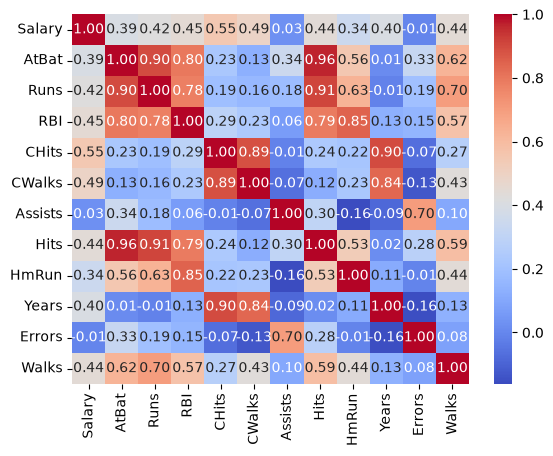
We now continue to prepare our data by defining target and features and split it into training and test set:
from sklearn.model_selection import train_test_split

y = hitters_subset["Salary"]
X = hitters_subset.drop(columns=["Salary"])

X_train, X_test, y_train, y_test = train_test_split(X, y, test_size=0.3, random_state=42)
Great! We are now ready for using the data in our regression models.
Ridge Regression
The loss function for ridge regression is defined as:
Where:
is the number of observations
is the number of predictors
is the target for observation is the row vector of features for observation
are the regression coefficients
is the regularization strength
Combined:
is the residual sum of squares (RSS)
is the L2 penalty on the coefficients (the intercept is not penalized)
We can implement Ridge regression as follows:
Step 1: We first standardize the predictors as ridge regression is sensitive to scaling. This can be done by using e.g. StandardScaler from scikit-learn:
from matplotlib import pyplot as plt
from sklearn.preprocessing import StandardScaler

scaler = StandardScaler() # Scale predictors to mean=0 and std=1
X_train_scaled = scaler.fit_transform(X_train)
X_test_scaled = scaler.transform(X_test)
Step 2: Next, we set up a range of values for λ. Good values can lie anywhere between very small and very large, so we test 100 values between 0.01 and 10,000 that are evenly spaced on a log scale:
import numpy as np

lambda_range = np.logspace(-2, 4, 100)
Step 3: For each lambda, we will perform ridge regression on the training data. Cross-validation is then used to identify the optimal lambda that minimizes prediction error:
from sklearn.linear_model import RidgeCV
import pandas as pd

# Get the optimal lambda
ridge_cv = RidgeCV(alphas=lambda_range, cv=5)
ridge_cv.fit(X_train_scaled, y_train)

print(f"Optimal alpha: {ridge_cv.alpha_}")

# Get training R²
train_score_ridge= ridge_cv.score(X_train_scaled, y_train)
print(f"Training R²: {train_score_ridge}")
Optimal alpha: 100.0
Training R²: 0.4602782368374775
We can then inspect the coefficients of the regression model:
# Put the coefficients into a nicely formatted df for visualization
coef_table = pd.DataFrame({
    'Predictor': X_train.columns,
    'Beta': ridge_cv.coef_
})

coef_table = coef_table.reindex(coef_table['Beta'].abs().sort_values(ascending=False).index)
print(coef_table)
Predictor Beta
3 CHits 75.496776
6 Hits 56.284067
4 CWalks 48.245080
8 Years 41.904244
1 Runs 32.287559
7 HmRun 30.376020
2 RBI 29.545059
10 Walks 29.261608
0 AtBat 22.857245
9 Errors -7.097005
5 Assists -6.945251
Step 4: Finally, we can evaluate the model on the testing data to assess its ability for generalization:
test_score_ridge = ridge_cv.score(X_test_scaled, y_test)

print(f"Test R²: {test_score_ridge}")
Test R²: 0.2917715098347792
Additional visualization: To get a better intuition about how different lambda values affect the beta estimates, we can plot them for each model. The dashed line marks the λ chosen by cross-validation:
from sklearn.linear_model import Ridge

coefs = []
for a in lambda_range:
    ridgereg = Ridge(alpha=a)
    ridgereg.fit(X_train_scaled, y_train)
    coefs.append(ridgereg.coef_)

# Plot
fig, ax = plt.subplots()
ax.plot(lambda_range, coefs)
ax.axvline(ridge_cv.alpha_, color="k", ls="--")
ax.set(title="Ridge coefficients", xlabel="Lambda (log scale)", ylabel="Beta", xscale="log");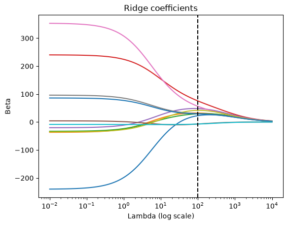
Lasso Regression
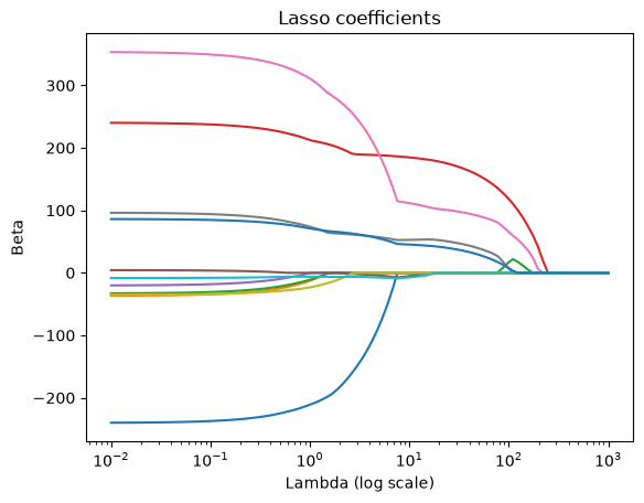
In contrast to ridge regression, lasso regression can set some coefficients exactly to zero, which removes these predictors from the model. The loss function for lasso is given as:
Where:
is the residual sum of squares (RSS)
is the L1 penalty on the coefficients
You can see, that the concept is nearly identical, with the only difference being the form of the penalty term. Lasso uses the L1 norm () while Ridge uses the L2 norm (). Because of this geometric difference in the penalty, Lasso can produce sparse models by zeroing out irrelevant features, whereas Ridge keeps all predictors in the model but with smaller weights. Both balance the trade‐off between model fit (the RSS term) and complexity via the tuning parameter λ, typically chosen by cross‐validation.
Interactive: watch the coefficients shrink
The two path plots show all coefficients at once, which is informative but hard to read. Below, drag the slider to pick a single value of λ and compare the Ridge and Lasso models side by side: both their coefficients and what the shrinkage costs (or gains) you on the test set.
Source
import numpy as np
import plotly.graph_objects as go
import plotly.io as pio
from sklearn.linear_model import Ridge, Lasso

# Neutral template that stays legible in light and dark mode
tpl = pio.templates["plotly_white"]
tpl.layout.paper_bgcolor = "rgba(0,0,0,0)"
tpl.layout.plot_bgcolor = "rgba(128,128,128,0.08)"
tpl.layout.font.color = "#888888"
pio.templates["psy300"] = tpl
pio.templates.default = "psy300"

features = list(X_train.columns)
lambdas = np.round(np.logspace(-2, 2.4, 25), 3)

traces, steps, info = [], [], []
for i, lam in enumerate(lambdas):
    ridge = Ridge(alpha=lam).fit(X_train_scaled, y_train)
    lasso = Lasso(alpha=lam, max_iter=10000).fit(X_train_scaled, y_train)

    traces.append(go.Bar(x=features, y=ridge.coef_, name="Ridge",
                         marker_color="#4c72b0", visible=False))
    traces.append(go.Bar(x=features, y=lasso.coef_, name="Lasso",
                         marker_color="#dd8452", visible=False))

    info.append(
        f"λ = {lam:g}   |   "
        f"Ridge test R² = {ridge.score(X_test_scaled, y_test):.3f}   |   "
        f"Lasso test R² = {lasso.score(X_test_scaled, y_test):.3f}   |   "
        f"Lasso coefficients set to zero: {int(np.sum(lasso.coef_ == 0))}/{len(features)}"
    )

traces[0].visible = True
traces[1].visible = True

# Fix the y-axis to the coefficients at the smallest λ (with 10% margin)
initial_coefs = np.concatenate([traces[0].y, traces[1].y])
y_range = [1.1 * min(initial_coefs.min(), 0), 1.1 * max(initial_coefs.max(), 0)]

for i, lam in enumerate(lambdas):
    vis = [False] * len(traces)
    vis[2 * i] = vis[2 * i + 1] = True
    steps.append(dict(method="update", label=f"{lam:g}",
                      args=[{"visible": vis},
                            {"annotations": [dict(x=0.5, y=1.14, xref="paper", yref="paper",
                                                  text=info[i], showarrow=False,
                                                  font=dict(size=13), xanchor="center")]}]))

fig = go.Figure(data=traces)
fig.update_layout(
    barmode="group",
    sliders=[dict(active=0, currentvalue={"prefix": "Regularisation strength λ = "},
                  pad={"t": 40}, steps=steps)],
    annotations=[dict(x=0.5, y=1.14, xref="paper", yref="paper", text=info[0],
                      showarrow=False, font=dict(size=13), xanchor="center")],
    yaxis_title="Coefficient (standardised predictors)",
    yaxis_range=y_range,
    margin=dict(l=10, r=10, t=90, b=20),
    height=470,
)
figTwo behaviours become obvious as you move the slider to the right:
Ridge shrinks every coefficient smoothly towards zero, but never quite reaches it. All predictors stay in the model.
Lasso switches predictors off one after another. The counter above the plot shows how many coefficients are exactly zero. The penalty performs feature selection as a side effect.
Why Ridge and Lasso Behave Differently: The Budget
There is a second way to look at the penalty. Instead of adding it to the RSS, we can give the model a fixed budget for the size of its coefficients. We then look for the coefficients with the smallest RSS that stay within this budget:
Lasso:
Ridge:
Both views are equivalent: a large λ corresponds to a small budget , and λ = 0 to an unlimited budget.
With only two coefficients, we can draw the budget as an area. Let’s take a budget of and look at the points that use it up completely:
Lasso: all points with , for example , , , or . Within each quadrant, these points lie on a straight line (e.g. when both are positive). The four lines form a diamond with its corners on the axes.
Ridge: all points with . By Pythagoras, these are exactly the points at distance 1 from the origin, so they form a circle.
Everything inside the diamond or the circle stays within the budget:
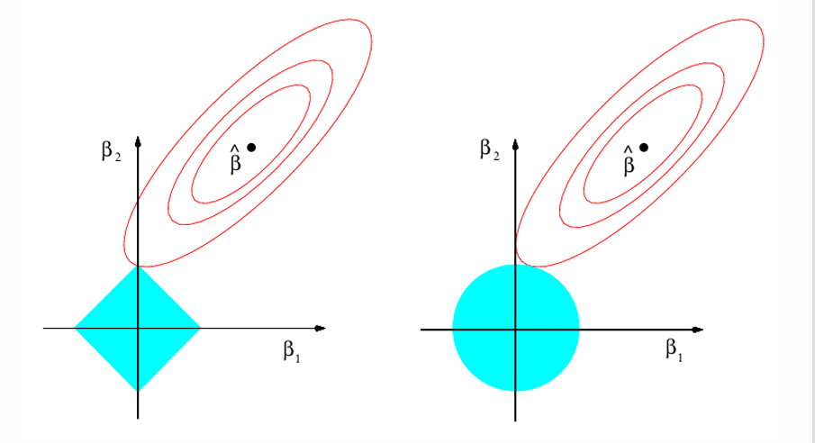
Figure 1:The budget for Lasso (left) and Ridge (right) regression. Figure from James et al., An Introduction to Statistical Learning, Figure 6.7.
The blue area contains all combinations of and that fit into the budget. For Lasso, it is a diamond, for Ridge a circle.
is the least squares solution, the combination with the smallest RSS. It lies outside the blue area, so we cannot afford it.
The red ellipses connect combinations with the same RSS. The further away from , the larger the RSS.
The solution is the point within the budget that has the smallest RSS. We find it by growing the ellipses around until they first touch the blue area. For Lasso, this often happens at a corner of the diamond. The corners lie on the axes, where one of the coefficients is exactly zero (here ). The circle has no corners, so Ridge usually ends up at a point where both coefficients are non-zero, just smaller. With many predictors, the diamond has many corners and edges, so Lasso solutions with several zeros are common.
Elastic Net Regression
Neither Ridge nor Lasso will universally be better than the other. The main difference between them is the coefficient selection:
Lasso tends to shrink some coefficients all the way to zero, effectively performing feature selection by excluding less relevant variables.
Ridge also shrinks coefficients toward zero, but does not eliminate any completely. Instead of selecting variables, it distributes the effect across all features.
Another point to note is their response to multicollinearity:
Ridge shares the weight among collinear features, keeping them all (shrink but don’t zero)
Lasso chooses a subset (often just one) from each collinear group and zeroes out the rest
This is where elastic net regression comes into play. Elastic net is a combination of Ridge and Lasso:
Here, the mixing parameter determines how much weight to give each penalty: when you recover pure Lasso (only an L1 penalty), and when you recover pure Ridge (only an L2 penalty); values in between blend the two. By combining these penalties, Elastic Net can both shrink coefficients (like Ridge) and select variables (like Lasso), while also tending to select or drop groups of correlated features together. In practice, you tune both λ (overall regularization strength) and via cross-validation to find the best compromise between bias, variance, and sparsity for your particular dataset.
As a summary, we can look at the coefficients estimated by all introduced methods, each with its λ chosen by cross-validation:
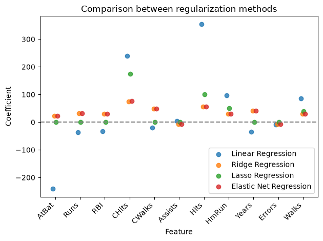
Look at AtBat and Hits: linear regression gives one a large negative and the other a large positive coefficient. The two predictors are correlated at 0.96, so OLS can trade one off against the other, and the estimates become unstable. All three regularized models keep both coefficients small. Elastic Net chose the smallest mixing ratio we offered (l1_ratio=0.1), so it behaves almost exactly like Ridge here, and its coefficients are nearly identical to the Ridge coefficients.
But which model predicts best? Let’s compare them on the test set:
models = {"Linear regression": lr, "Ridge": ridge_cv, "Lasso": lasso_cv, "Elastic net": enet_cv}

comparison = pd.DataFrame({
    "Test R²": [m.score(X_test_scaled, y_test) for m in models.values()],
    "Non-zero coefficients": [np.sum(m.coef_ != 0) for m in models.values()],
}, index=models.keys())

comparison.round(3)On this test set, plain linear regression actually performs best. With 184 training observations and only 11 predictors, OLS does not overfit much, so there is little variance that regularization could remove. Regularization pays off when there are many predictors relative to the number of observations, or when we want stable coefficients despite strongly correlated predictors. Lasso still offers something here: it reaches a test R² of 0.32 with only 4 of the 11 predictors.
Now it’s your turn: head to the exercise section for Exercise 2, in which you will implement a Lasso model.